
6.1. Thiết kế pipeline
Đầu tiên chúng ta sẽ cần import các packages cần thiết. Hầu hết các project machine learning đều yêu cầu sử dụng 4 packages chính là numpy, pandas (đọc, ghi và biến đổi dữ liệu), matplotlib (biểu đồ hoá) và đặc biệt là sklearn (xây dựng mô hình). Để import các package chính thì chúng ta có thể sử dụng câu lệnh import package as alias, câu lệnh này sẽ import một package có tên là package và gán cho nó một cái tên ngắn gọn là alias trong toàn bộ file xử lý. Hoặc nếu chỉ muốn import một hàm hoặc class trong package thì bạn sử dụng câu lệnh from package.module import class_or_funct. Câu lệnh này sẽ import một class hoặc hàm số là class_or_funct bên trong package.module.
#from google.colab import drive
#import os

#drive.mount('/content/gdrive')
#os.chdir('gdrive/MyDrive/mybook')

import pandas as pd
import numpy as np
import seaborn as sns
import matplotlib.pyplot as plt
from sklearn.compose import ColumnTransformer
from sklearn.naive_bayes import GaussianNB
from sklearn.linear_model import LogisticRegression
from sklearn.neighbors import KNeighborsClassifier
from sklearn.svm import LinearSVC
from sklearn.neural_network import MLPClassifier
from sklearn.ensemble import GradientBoostingClassifier
from sklearn.ensemble import RandomForestClassifier
from sklearn.impute import KNNImputer, SimpleImputer
from sklearn.metrics import accuracy_score
from sklearn.model_selection import train_test_split
from sklearn.pipeline import Pipeline
from sklearn.model_selection import cross_val_score
from sklearn.metrics import fbeta_score
from sklearn.metrics import make_scorer
from sklearn.model_selection import cross_val_score
from sklearn.model_selection import RepeatedStratifiedKFold
from sklearn.preprocessing import OneHotEncoder, MinMaxScaler
6.1.1. Tìm hiểu về bộ dữ liệu German credit
German credit là bộ dữ liệu về lịch sử tín dụng của 1000 tài khoản khác nhau. Mục tiêu của chúng ta là dựa vào lịch sử tín dụng này để dự đoán khả năng khách hàng sẽ trả nợ hay không. Bộ dữ liệu bao gồm 20 biến đầu vào trong đó có 7 biến liên tục (numeric) và 13 biến phân loại (category). Nội dung của các biến từ 1 đến 20 lần lượt như sau:
Trạng thái tài khoản hiện có.
Kỳ hạn theo tháng (Duration)
Lịch sử tín dụng
Mục đích
Dư nợ tín dụng (Credit amount)
Tài khoản tiết kiệm (Savings account)
Số năm làm việc liên tục gần nhất tới thời điểm hiện tại
Tỷ lệ trả góp (Installment rate) theo thu nhập khả dụng
Giới tính và trạng thái hôn nhân
Những người nợ khác
Thời gian cư trú tại nơi ở hiện tại
Bất động sản
Tuổi
Trả góp khác
Nhà ở
Số lượng khoản vay tại ngân hàng
Nghề nghiệp
Số người phụ thuộc
Điện thoại
Có phải là lao động nước ngoài
Biến mục tiêu (cột response ở vị trí cuối cùng) có giá trị 1 cho khách hàng Good và 2 cho khách hàng Bad. Khách hàng Good là khác hàng vỡ nợ và chúng ta còn gọi là Negative Class trong khi khách hàng Bad là trường hợp ngược lại và là Positive class.
Đây là bộ dữ liệu mất cân bằng khi nhãn Good (Negative) chiếm 70% và nhãn Bad chỉ 30% (Positive). Tiếp theo ta sẽ đọc vào khảo sát bộ dữ liệu này.
import pandas as pd

df = pd.read_csv("http://archive.ics.uci.edu/ml/machine-learning-databases/statlog/german/german.data",
                 header=None, names=['StaAcc', 'DuMon', 'CredHis', 'Purpose', 'CredAmt', 'SavAcc', \
                                     'PreEmpl', 'InsRt', 'PerSta', 'OthDebtor', 'PreRe', 'Property', \
                                     'Age', 'IntPla', 'Housing', 'ExstCredit', 'Job', 'NoMain', 'Phone', 'ForWorker', "Response"],
                 index_col=None, sep=" ")
df.head()
| StaAcc | DuMon | CredHis | Purpose | CredAmt | SavAcc | PreEmpl | InsRt | PerSta | OthDebtor | ... | Property | Age | IntPla | Housing | ExstCredit | Job | NoMain | Phone | ForWorker | Response | |
|---|---|---|---|---|---|---|---|---|---|---|---|---|---|---|---|---|---|---|---|---|---|
| 0 | A11 | 6 | A34 | A43 | 1169 | A65 | A75 | 4 | A93 | A101 | ... | A121 | 67 | A143 | A152 | 2 | A173 | 1 | A192 | A201 | 1 |
| 1 | A12 | 48 | A32 | A43 | 5951 | A61 | A73 | 2 | A92 | A101 | ... | A121 | 22 | A143 | A152 | 1 | A173 | 1 | A191 | A201 | 2 |
| 2 | A14 | 12 | A34 | A46 | 2096 | A61 | A74 | 2 | A93 | A101 | ... | A121 | 49 | A143 | A152 | 1 | A172 | 2 | A191 | A201 | 1 |
| 3 | A11 | 42 | A32 | A42 | 7882 | A61 | A74 | 2 | A93 | A103 | ... | A122 | 45 | A143 | A153 | 1 | A173 | 2 | A191 | A201 | 1 |
| 4 | A11 | 24 | A33 | A40 | 4870 | A61 | A73 | 3 | A93 | A101 | ... | A124 | 53 | A143 | A153 | 2 | A173 | 2 | A191 | A201 | 2 |
5 rows × 21 columns
Các trường dữ liệu và định dạng
df.info()
<class 'pandas.core.frame.DataFrame'>
RangeIndex: 1000 entries, 0 to 999
Data columns (total 21 columns):
 #   Column      Non-Null Count  Dtype
---  ------      --------------  -----
 0   StaAcc      1000 non-null   object
 1   DuMon       1000 non-null   int64
 2   CredHis     1000 non-null   object
 3   Purpose     1000 non-null   object
 4   CredAmt     1000 non-null   int64
 5   SavAcc      1000 non-null   object
 6   PreEmpl     1000 non-null   object
 7   InsRt       1000 non-null   int64
 8   PerSta      1000 non-null   object
 9   OthDebtor   1000 non-null   object
 10  PreRe       1000 non-null   int64
 11  Property    1000 non-null   object
 12  Age         1000 non-null   int64
 13  IntPla      1000 non-null   object
 14  Housing     1000 non-null   object
 15  ExstCredit  1000 non-null   int64
 16  Job         1000 non-null   object
 17  NoMain      1000 non-null   int64
 18  Phone       1000 non-null   object
 19  ForWorker   1000 non-null   object
 20  Response    1000 non-null   int64
dtypes: int64(8), object(13)
memory usage: 164.2+ KB
Đây là bộ dữ liệu có chất lượng khá tốt, không có missing value ở các biến.
Thống kê mô tả
df.describe()
| DuMon | CredAmt | InsRt | PreRe | Age | ExstCredit | NoMain | Response | |
|---|---|---|---|---|---|---|---|---|
| count | 1000.000000 | 1000.000000 | 1000.000000 | 1000.000000 | 1000.000000 | 1000.000000 | 1000.000000 | 1000.000000 |
| mean | 20.903000 | 3271.258000 | 2.973000 | 2.845000 | 35.546000 | 1.407000 | 1.155000 | 1.300000 |
| std | 12.058814 | 2822.736876 | 1.118715 | 1.103718 | 11.375469 | 0.577654 | 0.362086 | 0.458487 |
| min | 4.000000 | 250.000000 | 1.000000 | 1.000000 | 19.000000 | 1.000000 | 1.000000 | 1.000000 |
| 25% | 12.000000 | 1365.500000 | 2.000000 | 2.000000 | 27.000000 | 1.000000 | 1.000000 | 1.000000 |
| 50% | 18.000000 | 2319.500000 | 3.000000 | 3.000000 | 33.000000 | 1.000000 | 1.000000 | 1.000000 |
| 75% | 24.000000 | 3972.250000 | 4.000000 | 4.000000 | 42.000000 | 2.000000 | 1.000000 | 2.000000 |
| max | 72.000000 | 18424.000000 | 4.000000 | 4.000000 | 75.000000 | 4.000000 | 2.000000 | 2.000000 |
Kết quả thống kê mô tả sơ bộ trên các biến numeric cho thấy các biến khác biệt nhau về đơn vị lớn. Trung bình thấp nhất là 1.155 và cao nhất lên tới 3271.258. Như vậy khả năng cao chúng ta sẽ cần phải chuẩn hoá các biến để loại bỏ sự khác biệt về đơn vị trước khi xây dựng mô hình.
Phân phối của các biến
Chúng ta không nên tin tưởng hoàn toàn vào thống kê mô tả mà cần nhìn trực tiếp vào hình dạng phân phối của các biến. Điều này nhằm tránh những sai sót khi đánh giá về tính chất của biến khi chúng khác biệt xa nhau về phân phối. Điều này đã được giải thích trong ví dụ phân phối chú khủng long.
Chúng ta có thể dùng biểu đồ density kết hợp với histogram để tìm ra phân phối của biến.
Đối với biến liên tục.
import seaborn as sns
import warnings
warnings.simplefilter(action='ignore', category=FutureWarning)

numeric_cols = df.select_dtypes(include=['float','int']).columns

def _plot_numeric_classes(df, col, bins=10, hist=True, kde=True):
    sns.distplot(df[col],
                 bins = bins,
                 hist = hist,
                 kde = kde)

def _distribution_numeric(df, numeric_cols, row=3, col=3, figsize=(20, 15), bins = 10):
    '''
    numeric_cols: list các tên cột
    row: số lượng dòng trong lưới đồ thị
    col: số lượng cột trong lưới đồ thị
    figsize: kích thước biểu đồ
    bins: số lượng bins phân chia trong biểu đồ distribution
    '''
    print('number of numeric field: ', len(numeric_cols))
    assert row*(col-1) < len(numeric_cols)
    plt.figure(figsize = figsize)
    plt.subplots_adjust(left=None, bottom=None, right=None, top=None, wspace=0.2, hspace=0.5)
    for i in range(1, len(numeric_cols)+1, 1):
      try:
        plt.subplot(row, col, i)
        _plot_numeric_classes(df, numeric_cols[i-1], bins = bins)
        plt.title(numeric_cols[i-1])
      except:
        print('Error {}'.format(numeric_cols[i-1]))
        break

_distribution_numeric(df, numeric_cols)
number of numeric field: 8
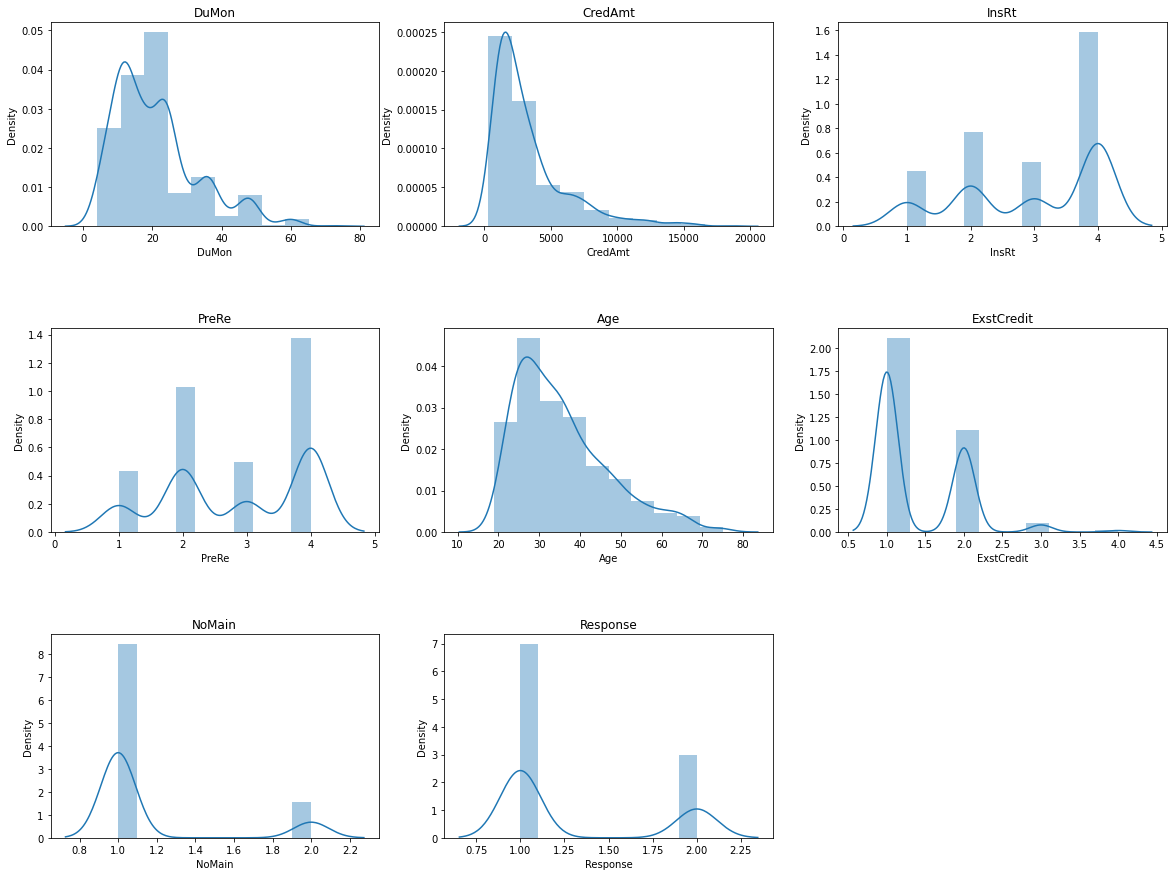
Ta nhận thấy một số biến thực chất là biến thứ bậc khi các giá trị chỉ rơi vào một tập giá trị nhất định, chẳng hạn như biến PreReg chỉ nhận các giá trị 1, 2, 3, 4. Khi nhìn vào biểu đồ phân phối của biến ta có thể nhận định đâu là miền mà các biến có mật độ tập trung cao và thấp? Kết hợp với kinh nghiệm business để đánh giá phân phối của biến có phù hợp với thực tế hay không? Đối với trường hợp có quá nhiều biến cần kiểm tra thì chúng ta có thể đối chiếu với phân phối của dữ liệu lịch sử để xem xét những thay đổi của biến. Điều này rất quan trọng vì sự thay đổi của biến sẽ ảnh hưởng trực tiếp tới đầu ra của mô hình.
Tương tự đối với biến phân loại chúng ta sẽ thống kê được tần suất giá trị của các nhãn trong một biến.
# Đối với biến phân loại
cate_cols = df.select_dtypes('O').columns

def _plot_bar_classes(df, cols):
    df[cols].value_counts().plot.bar()

def _distribution_cate(df, cate_cols, row = 1, col = 2, figsize = (20, 5)):
  '''
  cate_cols: list các tên cột
  row: số lượng dòng trong lưới đồ thị
  col: số lượng cột trong lưới đồ thị
  figsize: kích thước biểu đồ
  '''
  print('number of category field: ', len(cate_cols))
  plt.figure(figsize = figsize)
  plt.subplots_adjust(left=None, bottom=None, right=None, top=None, wspace=0.2, hspace=0.5)
  for i in range(1, len(cate_cols)+1, 1):
    try:
      plt.subplot(row, col, i)
      _plot_bar_classes(df, cate_cols[i-1])
      plt.title(cate_cols[i-1])
    except:
      break

_distribution_cate(df, cate_cols, row = 4, col = 4, figsize = (30, 16))
number of category field: 13
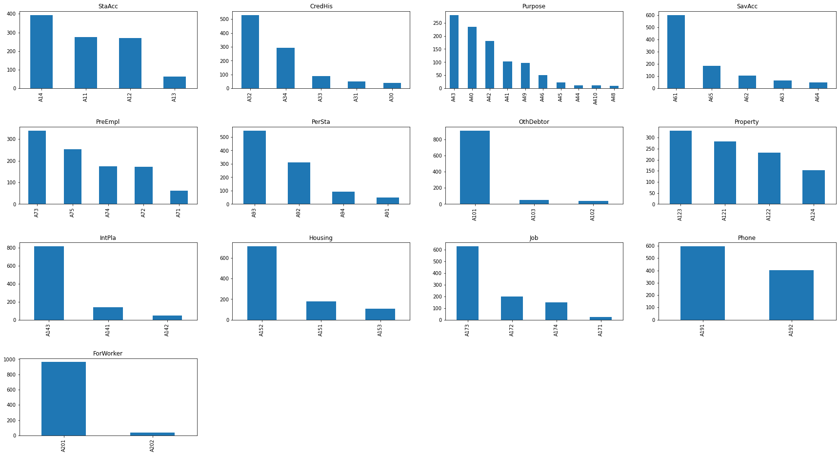
Ta nhận thấy có nhiều nhãn trong biến phân loại có số lượng quan sát rất ít. Theo kinh nghiệm thì các nhãn thiểu số lại có thể là đặc trưng riêng của một nhãn đầu ra. Vì thế chúng ta có thể khảo sát thêm tỷ lệ giữa GOOD/BAD cách biệt như thế nào ở những nhãn này. Kết quả đánh giá chúng có thể giúp ta đưa ra một số kết luận hữu ích đối với phân loại nhãn.
6.1.2. Phân chia tập train/val/test
Hầu hết các mô hình machine learning đều yêu cầu việc phân chia tập train/test. Tiếp theo đó chúng ta sẽ tách một phần nhỏ từ tập train thành tập validation dùng để đánh giá mô hình. Một số bộ dữ liệu lớn chúng ta còn tách thành tập train/dev/test trong đó:
Tập train: Huấn luyện mô hình. Chúng ta có thể huấn luyện mô hình trên tập train theo phương pháp cross validation. Khi đó tập validation sẽ được tách ra từ tập train để đánh giá độc lập hiệu suất của mô hình và kiểm tra các hiện tượng overfitting và underfitting.
Tập test: Đánh giá lại mô hình trên những dữ liệu mới và khắc phục các sự cố mô hình như overfitting, underfitting.
Tập dev: Đánh giá mô hình để đưa ra các quyết định lựa chọn siêu tham số phù hợp cho từng lớp mô hình.
Mục đích của tập train là huấn luyện mô hình nên tập train cần chiếm tỷ lệ lớn để giúp mô hình học bao quát được các trường hợp của dữ liệu. Tập validation là tập dữ liệu sử dụng để đánh giá lại mô hình xem có xảy ra các hiện tượng overfitting và underfitting hay không? Những hiện tượng này cần được khắc phục nhằm giúp mô hình dự báo tốt hơn trên dữ liệu thực tế.
Chúng ta thắc mắc nếu đã có tập validation thì tại sao lại cần thêm tập test? Tập test là một tập được lựa chọn sao cho phân phối và tính chất giống với dữ liệu thực tế nhất. Mục tiêu của tập này là để kiểm tra hiệu năng của mô hình nếu triển khai trên production. Thông thường kích thước tập test được lấy bằng tập validation. Để lựa chọn mô hình nào tốt nhất chúng ta sẽ căn cứ trên kết quả đánh giá trên tập test.
Tỷ lệ phân chia train/test khá đa dạng và không có qui định cụ thể. Theo kinh nghiệm, chúng ta có thể lấy theo các tỷ lệ 50:50 hoặc 70:30 nếu dữ liệu dồi dào, 80:20 hoặc 90:10 nếu dữ liệu ít.
Để phân chia dữ liệu chúng ta dùng hàm train_test_split(). Lựa chọn stratify=df['Response'] để giúp cân bằng tỷ lệ Good/Bad trên cả train và test.
from sklearn.model_selection import train_test_split

# Chia train/test theo tỷ lệ 80:20.
df_train, df_test = train_test_split(df, test_size=0.2, stratify = df['Response'])
X_train = df_train.copy()
y_train = X_train.pop("Response")

X_test = df_test.copy()
y_test = X_test.pop("Response")
print(X_train.shape, y_train.shape)
print(X_test.shape, y_test.shape)
(800, 20) (800,)
(200, 20) (200,)
Tập validation sẽ được trích từ tập train ở trên theo tỷ lệ train/test=80/20. Cách chia này có thể cố định một lần hoặc thực hiện cross validation bằng cách chia thành K-Fold.
6.1.3. Preprocessing model
Bước tiếp theo là tiền xử lý dữ liệu. Ở bước này sẽ thực hiện các biến đổi chủ yếu nhằm biến dữ liệu thô chưa qua xử lý thành dữ liệu tinh có thể đưa vào mô hình huấn luyện. Trong sklearn hầu hết đã có sẵn những hàm chức năng giúp ta thực hiện các tiền xử lý dữ liệu một cách dễ dàng. Các xử lý chính bao gồm:
Số hoá cho các biến đầu vào dạng phân loại (dùng
OneHotEncoder).Xử lý missing data (dùng
SimpleImputer).Loại bỏ các outlier (dùng
MinMaxScaler).
Để kiểm soát các bước xử lý một cách tuần tự thì chúng ta sẽ thiết kế một pipeline khai báo các bước xử lý ở bên trong nó. Như vậy khi cần huấn luyện và dự báo chúng ta chỉ cần đưa vào dữ liệu thô vào pipeline để thu được đầu ra là dữ liệu tinh có thể huấn luyện và dự báo được.
6.1.4. Tách biệt xử lý cho biến liên tục và biến phân loại
Do các biến liên tục và biến phân loại có tính chất khác biệt nhau. Đối với biến liên tục thì có thể huấn luyện trực tiếp mô hình trên đó còn biến phân loại sẽ cần chúng ta mã hoá thành biến số học trước khi huấn luyện. Như vậy sẽ cần pipeline xử lý riêng cho từng loại biến. Để xây dựng pipeline trong sklearn chúng ta sử dụng hàm Pipeline(). Bên trong hàm này là một list gồm các steps xử lý theo tuần tự. Tiếp theo chúng ta sẽ thực hành thiết kế một pipeline mẫu cho bài toán này. Code mẫu cho bước này được tham khảo tại pipeline đơn giản cho cuộc thi Titanic.
# Lấy list names của các biến phân loại và biến liên tục.
cat_names = list(X_train.select_dtypes('object').columns)
num_names = list(X_train.select_dtypes(['float', 'int']).columns)
from sklearn.pipeline import Pipeline

# Pipeline xử lý cho biến phân loại
cat_pl= Pipeline(
    steps=[
        ('imputer', SimpleImputer(strategy='most_frequent')), # Xử lý missing data bằng cách thay thế most frequent
        ('onehot', OneHotEncoder()), # Biến đổi giá trị của biến phân loại thành véc tơ OneHot
    ]
)
# Pipeline xử lý cho biến liên tục
num_pl = Pipeline(
    steps=[
           ('imputer', KNNImputer(n_neighbors=7)), # Xử lý missing data bằng cách dự báo KNN với n=7.
           ('scaler', MinMaxScaler()) # Xử lý missing data bằng MinMax scaler
    ]
)
Các bạn nhận thấy các bước trong steps của Pipeline là một tuple gồm hai phần tử. Phần tử đầu tiên là tên của bước xử lý và phần tử thứ hai là phương pháp xử lý tương ứng. Việc đặt tên cho bước xử lý sẽ giúp ta nắm bắt được thứ tự và kiểm soát toàn bộ quá trình xử lý.
class ColumnTransformer trong sklearn là một phương pháp biến đổi được áp dụng trên các cột. Chúng ta có thể gộp chung hai biến đổi trên biến liên tục và phân loại như sau thông qua class này như sau:
from sklearn.compose import ColumnTransformer

preprocessor = ColumnTransformer(
    transformers=[
        ('num', num_pl, num_names), # áp dụng pipeline cho biến liên tục
        ('cat', cat_pl, cat_names), # áp dụng pipeline cho biến phân loại
    ]
)
Như vậy các biến liên tục được qui định trong list num_names sẽ áp dụng xử lý là pipeline num_pl và biến phân loại trong list cate_names sẽ áp dụng xử lý là pipeline cat_pl.
6.1.5. Pipeline hoàn chỉnh
Sau khi đã có Pipleline tiền xử lý dữ liệu hàn chỉnh thì chúng ta đã có thể thu được dữ liệu sạch ở đầu ra. Tiếp theo cần đưa dữ liệu đã làm sạch qua mô hình để huấn luyện. Cả hai bước tiền xử lý dữ liệu và huấn luyên mô hình có thể tiếp tục đóng gói trong một Pipeline như sau:
# Completed training pipeline
completed_pl = Pipeline(
    steps=[
            ("preprocessor", preprocessor),
            ("classifier", RandomForestClassifier())
    ]
)

# training
completed_pl.fit(X_train, y_train)

# accuracy
y_train_pred = completed_pl.predict(X_train)
print(f"Accuracy on train: {accuracy_score(list(y_train), list(y_train_pred)):.2f}")

y_pred = completed_pl.predict(X_test)
print(f"Accuracy on test: {accuracy_score(list(y_test), list(y_pred)):.2f}")
Accuracy on train: 1.00
Accuracy on test: 0.71
Như vậy chúng ta đã hoàn thiện một Pipeline đơn giản cho mô hình phân loại khả năng trả nợ. Mô hình có độ chính xác trên tập train là 100% và trên tập test là 77% cho thấy có hiện tượng overfitting. Để khắc phục overfitting chúng ta có thể thực hiện cross validation.
6.2. Đánh giá cheó (cross validation)
Đánh giá chéo là một thủ tục lấy mẫu được sử dụng để đánh giá các mô hình machine learning trong quá trình huấn luyện. Cụ thể trong đánh giá chéo (cross validation) chúng ta phân chia dữ liệu thành k-folds không chồng lấn, có kích thước bằng nhau. Ở mỗi lượt huấn luyện ta sẽ lựa chọn ra (k-1) folds để huấn luyện và fold còn lại để kiểm định. Như vậy đánh giá chéo sẽ đánh giá được khả năng dự báo của mô hình đối với dữ liệu mà nó chưa nhìn thấy. Căn cứ vào kết quả trên toàn bộ các folds thì chúng ta có thể rút ra kết luận về trung bình, phương sai của các thước đo đánh giá hiệu suất của mô hình và đưa ra đánh giá sơ bộ về sức mạnh của chúng.

Hình 1: Source - cross validation, sklearn. Quá trình phân chia dữ liệu, huấn luyện và đánh giá mô hình dựa trên đánh giá chéo.
6.2.1. Lựa chọn thước đo mô hình
Lựa chọn thước đo cho mô hình là một công việc khó vì nó đòi hỏi người xây dựng mô hình phải hiểu sâu về vấn đề mình đang giải quyết và đồng thời có kiến thức chuyên môn về mô hình.
Trong trường hợp là người chưa có kinh nghiệm bạn có thể lựa chọn các thước đo mô hình thông dụng của bài toán dự báo và bài toán phân loại như bên dưới.
6.2.1.1.Thước đo sơ bộ cho bài toán dự báo
Trong bài toán dự báo thì chúng ta muốn sai số giữa giá trị dự báo và giá trị thực tế là nhỏ nhất nên MSE (mean squared error), RMSE (root mean squared error), MAE (mean absolute error) hoặc MAPE (mean absolute percentage error) thường được lựa chọn.
Nhìn vào công thức bạn cũng có thể hình dung sơ bộ ý nghĩa của các chỉ số này rồi chứ?
MSE: Trung bình tổng bình phương sai số giữa giá trị dự báo và thực tế.
RMSE: Khai căn bậc hai của MSE và nó đại diện cho độ lệch giữa giá trị dự báo và thực tế.
MAE: Trung bình trị tuyệt đối của sai số giữa giá trị dự báo và thực tế.
MAPE: Trung bình của tỷ lệ phần trăm sai số tuyệt đối giữa giá trị dự báo và thực tế.
6.2.1.2. Thước đo sơ bộ cho bài toán phân loại
Lấy ví dụ một bài toán phân loại nhị phân có bảng chéo thống kê kết quả giữa thực tế và dự báo như sau:
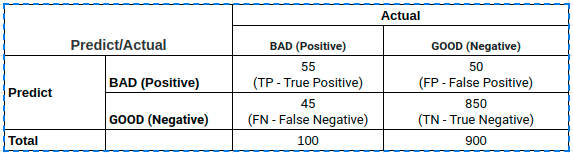
Các chỉ số TP, FP, TN, FN lần lượt có ý nghĩa là :
TP (True Positive): Tổng số trường hợp dự báo khớp Positive.
TN (True Negative): Tổng số trường hợp dự báo khớp Negative.
FP (False Positive): Tổng số trường hợp dự báo các quan sát thuộc nhãn Negative thành Positive. Những sai lầm của False Positive tương ứng với sai lầm loại I (type I error), chấp nhận một điều sai. Thực tế cho thấy sai lầm loại I thường gây hậu quả nghiêm trọng hơn so với sai lầm loại II được tìm hiểu bên dưới.
FN (False Negative): Tổng số trường hợp dự báo các quan sát thuộc nhãn Positive thành Negative. Trong trường hợp này chúng ta mắc sai lầm loại II (type II error), bác bỏ một điều đúng.
Đối với bài toán phân loại thì ta quan tâm tới độ chính xác dự báo trên toàn bộ bộ dữ liệu là bao nhiêu? do đó thước đo phổ biến nhất là accuracy.
Bài tập: Bạn hãy giải thích vì sao trong trường hợp mất cân bằng dữ liệu thì accuracy không còn là thước đo mô hình tốt?
Trong tính huống mô hình bị mất cân bằng thì accuracy không còn là thước đo tốt nên được thay thế bằng precision, recall.
Hai chỉ số này lần lượt giúp đánh giá tỷ lệ dự báo chính xác positive trên tổng số trường hợp được dự báo là positive và tỷ lệ dự báo chính xác positive trên thực tế. Thực sự rất khó để nói lựa chọn precision hay recall là tốt hơn nên chúng ta dùng f1-score là trung bình điều hoà đại diện cho cả precision và recall. Ngoài ra còn một số chỉ số nâng cao hơn cũng được lựa chọn để đánh giá sức mạnh phân loại như AUC, Gini Index, Cohen's Kappa tuy nhiên f1-score và accuracy theo mình nghĩ vẫn là hai chỉ số cơ bản nhất cho bài toán phân loại mà bạn cần nắm vững.
\(f_{\beta}\) là trường hợp tổng quát hơn của \(f_1\) khi ta coi mức độ quan trọng của recall bằng \(\beta\) lần precision.
Bộ dữ liệu german credit có tính chất mất cân bằng nên chúng ta sẽ lựa chọn f-score thay cho accuracy. Hơn nữa trong mô tả của bộ dữ liệu đã qui định:
It is worse to class a customer as good when they are bad (5), than it is to class a customer as bad when they are good (1).
Tức là một trường hợp False Negative có mức độ sai lầm bằng 5 trường hợp False Positive nên ta sẽ lựa chọn \(\beta^2=5\).
from sklearn.metrics import fbeta_score
from sklearn.metrics import make_scorer
import numpy as np

# Tính fbeta score
def fbeta(y_true, y_pred):
	return fbeta_score(y_true, y_pred, beta=np.sqrt(5))
6.2.1.3. Thực hiện cross validation
Để thực hiện cross validation chúng ta sử dụng class RepeatedStratifiedKFold() với n_splits là số lần chia dữ liệu và n_repeates là số lần lặp lại quá trình cross validation. Như vậy chúng ta sẽ có tổng cộng n_splits x n_repeats = 30 lượt đánh giá dữ liệu.
Hàm cross_val_score() sẽ được sử dụng để tính toán thước đo mô hình trên các lượt huấn luyện.
from sklearn.model_selection import cross_val_score, RepeatedStratifiedKFold

# Xác định KFold
cv = RepeatedStratifiedKFold(n_splits=10, n_repeats=3, random_state=1)
# Xác định metric cho mô hình
metric = make_scorer(fbeta)
# Đánh giá mô hình
scores = cross_val_score(completed_pl, X_train, y_train, scoring=metric, cv=cv, n_jobs=-1)
print('Mean Fbeta: {:.03f} {:.03f}'.format(np.mean(scores), np.std(scores)))
Mean Fbeta: 0.895 0.034
6.2.2. Đánh giá nhiều mô hình
Chúng ta có thể thực hiện vòng lặp để đánh giá chéo nhiều lớp mô hình khác nhau. Sau đó so sánh phân phối điểm thu được của những lớp mô hình này để tìm ra đâu là mô hình có score lớn nhất.
from sklearn.ensemble import RandomForestClassifier
from sklearn.naive_bayes import GaussianNB
from sklearn.linear_model import LogisticRegression
from sklearn.neighbors import KNeighborsClassifier
from sklearn.neural_network import MLPClassifier
# list các mô hình được lựa chọn
models = [GaussianNB(), LogisticRegression(), KNeighborsClassifier(), MLPClassifier(), RandomForestClassifier()]

# Xác định KFold
cv = RepeatedStratifiedKFold(n_splits=10, n_repeats=3, random_state=1)

all_scores = []
# Đánh giá toàn bộ các mô hình trên tập K-Fold đã chia
for model in models:
  completed_pl = Pipeline(
    steps=[("preprocessor", preprocessor), ('classifier', model)]
  )

  scores = cross_val_score(completed_pl, X_train, y_train, scoring=metric, cv=cv, n_jobs=-1)
  all_scores.append(scores)
/home/khanh/miniconda3/envs/deepai-book/lib/python3.9/site-packages/sklearn/neural_network/_multilayer_perceptron.py:692: ConvergenceWarning: Stochastic Optimizer: Maximum iterations (200) reached and the optimization hasn't converged yet.
  warnings.warn(
/home/khanh/miniconda3/envs/deepai-book/lib/python3.9/site-packages/sklearn/neural_network/_multilayer_perceptron.py:692: ConvergenceWarning: Stochastic Optimizer: Maximum iterations (200) reached and the optimization hasn't converged yet.
  warnings.warn(
/home/khanh/miniconda3/envs/deepai-book/lib/python3.9/site-packages/sklearn/neural_network/_multilayer_perceptron.py:692: ConvergenceWarning: Stochastic Optimizer: Maximum iterations (200) reached and the optimization hasn't converged yet.
  warnings.warn(
/home/khanh/miniconda3/envs/deepai-book/lib/python3.9/site-packages/sklearn/neural_network/_multilayer_perceptron.py:692: ConvergenceWarning: Stochastic Optimizer: Maximum iterations (200) reached and the optimization hasn't converged yet.
  warnings.warn(
/home/khanh/miniconda3/envs/deepai-book/lib/python3.9/site-packages/sklearn/neural_network/_multilayer_perceptron.py:692: ConvergenceWarning: Stochastic Optimizer: Maximum iterations (200) reached and the optimization hasn't converged yet.
  warnings.warn(
/home/khanh/miniconda3/envs/deepai-book/lib/python3.9/site-packages/sklearn/neural_network/_multilayer_perceptron.py:692: ConvergenceWarning: Stochastic Optimizer: Maximum iterations (200) reached and the optimization hasn't converged yet.
  warnings.warn(
/home/khanh/miniconda3/envs/deepai-book/lib/python3.9/site-packages/sklearn/neural_network/_multilayer_perceptron.py:692: ConvergenceWarning: Stochastic Optimizer: Maximum iterations (200) reached and the optimization hasn't converged yet.
  warnings.warn(
/home/khanh/miniconda3/envs/deepai-book/lib/python3.9/site-packages/sklearn/neural_network/_multilayer_perceptron.py:692: ConvergenceWarning: Stochastic Optimizer: Maximum iterations (200) reached and the optimization hasn't converged yet.
  warnings.warn(
/home/khanh/miniconda3/envs/deepai-book/lib/python3.9/site-packages/sklearn/neural_network/_multilayer_perceptron.py:692: ConvergenceWarning: Stochastic Optimizer: Maximum iterations (200) reached and the optimization hasn't converged yet.
  warnings.warn(
/home/khanh/miniconda3/envs/deepai-book/lib/python3.9/site-packages/sklearn/neural_network/_multilayer_perceptron.py:692: ConvergenceWarning: Stochastic Optimizer: Maximum iterations (200) reached and the optimization hasn't converged yet.
  warnings.warn(
/home/khanh/miniconda3/envs/deepai-book/lib/python3.9/site-packages/sklearn/neural_network/_multilayer_perceptron.py:692: ConvergenceWarning: Stochastic Optimizer: Maximum iterations (200) reached and the optimization hasn't converged yet.
  warnings.warn(
/home/khanh/miniconda3/envs/deepai-book/lib/python3.9/site-packages/sklearn/neural_network/_multilayer_perceptron.py:692: ConvergenceWarning: Stochastic Optimizer: Maximum iterations (200) reached and the optimization hasn't converged yet.
  warnings.warn(
/home/khanh/miniconda3/envs/deepai-book/lib/python3.9/site-packages/sklearn/neural_network/_multilayer_perceptron.py:692: ConvergenceWarning: Stochastic Optimizer: Maximum iterations (200) reached and the optimization hasn't converged yet.
  warnings.warn(
/home/khanh/miniconda3/envs/deepai-book/lib/python3.9/site-packages/sklearn/neural_network/_multilayer_perceptron.py:692: ConvergenceWarning: Stochastic Optimizer: Maximum iterations (200) reached and the optimization hasn't converged yet.
  warnings.warn(
/home/khanh/miniconda3/envs/deepai-book/lib/python3.9/site-packages/sklearn/neural_network/_multilayer_perceptron.py:692: ConvergenceWarning: Stochastic Optimizer: Maximum iterations (200) reached and the optimization hasn't converged yet.
  warnings.warn(
/home/khanh/miniconda3/envs/deepai-book/lib/python3.9/site-packages/sklearn/neural_network/_multilayer_perceptron.py:692: ConvergenceWarning: Stochastic Optimizer: Maximum iterations (200) reached and the optimization hasn't converged yet.
  warnings.warn(
/home/khanh/miniconda3/envs/deepai-book/lib/python3.9/site-packages/sklearn/neural_network/_multilayer_perceptron.py:692: ConvergenceWarning: Stochastic Optimizer: Maximum iterations (200) reached and the optimization hasn't converged yet.
  warnings.warn(
/home/khanh/miniconda3/envs/deepai-book/lib/python3.9/site-packages/sklearn/neural_network/_multilayer_perceptron.py:692: ConvergenceWarning: Stochastic Optimizer: Maximum iterations (200) reached and the optimization hasn't converged yet.
  warnings.warn(
/home/khanh/miniconda3/envs/deepai-book/lib/python3.9/site-packages/sklearn/neural_network/_multilayer_perceptron.py:692: ConvergenceWarning: Stochastic Optimizer: Maximum iterations (200) reached and the optimization hasn't converged yet.
  warnings.warn(
/home/khanh/miniconda3/envs/deepai-book/lib/python3.9/site-packages/sklearn/neural_network/_multilayer_perceptron.py:692: ConvergenceWarning: Stochastic Optimizer: Maximum iterations (200) reached and the optimization hasn't converged yet.
  warnings.warn(
/home/khanh/miniconda3/envs/deepai-book/lib/python3.9/site-packages/sklearn/neural_network/_multilayer_perceptron.py:692: ConvergenceWarning: Stochastic Optimizer: Maximum iterations (200) reached and the optimization hasn't converged yet.
  warnings.warn(
/home/khanh/miniconda3/envs/deepai-book/lib/python3.9/site-packages/sklearn/neural_network/_multilayer_perceptron.py:692: ConvergenceWarning: Stochastic Optimizer: Maximum iterations (200) reached and the optimization hasn't converged yet.
  warnings.warn(
/home/khanh/miniconda3/envs/deepai-book/lib/python3.9/site-packages/sklearn/neural_network/_multilayer_perceptron.py:692: ConvergenceWarning: Stochastic Optimizer: Maximum iterations (200) reached and the optimization hasn't converged yet.
  warnings.warn(
/home/khanh/miniconda3/envs/deepai-book/lib/python3.9/site-packages/sklearn/neural_network/_multilayer_perceptron.py:692: ConvergenceWarning: Stochastic Optimizer: Maximum iterations (200) reached and the optimization hasn't converged yet.
  warnings.warn(
/home/khanh/miniconda3/envs/deepai-book/lib/python3.9/site-packages/sklearn/neural_network/_multilayer_perceptron.py:692: ConvergenceWarning: Stochastic Optimizer: Maximum iterations (200) reached and the optimization hasn't converged yet.
  warnings.warn(
/home/khanh/miniconda3/envs/deepai-book/lib/python3.9/site-packages/sklearn/neural_network/_multilayer_perceptron.py:692: ConvergenceWarning: Stochastic Optimizer: Maximum iterations (200) reached and the optimization hasn't converged yet.
  warnings.warn(
/home/khanh/miniconda3/envs/deepai-book/lib/python3.9/site-packages/sklearn/neural_network/_multilayer_perceptron.py:692: ConvergenceWarning: Stochastic Optimizer: Maximum iterations (200) reached and the optimization hasn't converged yet.
  warnings.warn(
/home/khanh/miniconda3/envs/deepai-book/lib/python3.9/site-packages/sklearn/neural_network/_multilayer_perceptron.py:692: ConvergenceWarning: Stochastic Optimizer: Maximum iterations (200) reached and the optimization hasn't converged yet.
  warnings.warn(
/home/khanh/miniconda3/envs/deepai-book/lib/python3.9/site-packages/sklearn/neural_network/_multilayer_perceptron.py:692: ConvergenceWarning: Stochastic Optimizer: Maximum iterations (200) reached and the optimization hasn't converged yet.
  warnings.warn(
/home/khanh/miniconda3/envs/deepai-book/lib/python3.9/site-packages/sklearn/neural_network/_multilayer_perceptron.py:692: ConvergenceWarning: Stochastic Optimizer: Maximum iterations (200) reached and the optimization hasn't converged yet.
  warnings.warn(
Tiếp theo ta sẽ vẽ biểu đồ phân phối score giữa các mô hình.
import matplotlib.pyplot as plt
model_names = ['GaussianNB', 'Logistic', 'KNN', 'MLP', 'RandomForest']

# Draw bboxplot
plt.figure(figsize=(16, 8))
plt.boxplot(all_scores)
plt.xlabel('Model', fontsize=16)
plt.ylabel('Score', fontsize=16)
plt.xticks(np.arange(len(model_names))+1, model_names, rotation=45, fontsize=16)
plt.title("Scores Metrics", fontsize=18)
Text(0.5, 1.0, 'Scores Metrics')
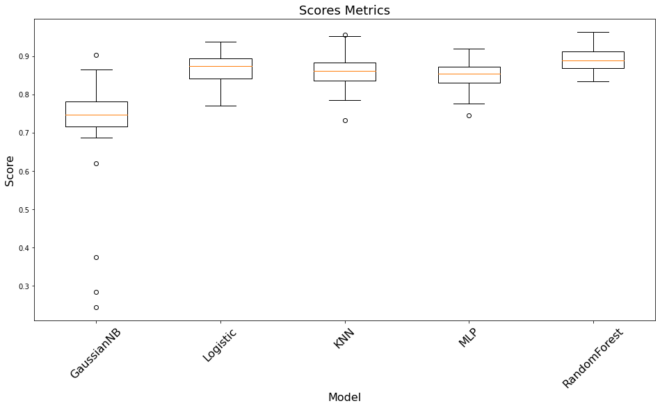
Nhìn vào biểu đồ ta có thể thấy RandomForest là thuật toán có độ chính xác cao nhất khi score giao động trong khoảng từ 0.83 đến 0.95 và trung bình đạt được khoảng 0.9 nên chúng ta sẽ lựa chọn lớp mô hình này để phát triển thành production.
6.3. GridSearch
GridSearch là một kỹ thuật giúp tìm kiếm tham số phù hợp cho mô hình đối với một bộ dữ liệu cụ thể. Trong sklearn chúng ta có thể sử dụng GridSearchCV để tạo không gian tham số. Để dễ hình dung hơn về GridSearch chúng ta hãy cùng áp dụng chúng trên bộ dữ liệu German Credit.
Đầu tiên chúng ta sẽ tạo ra một Class ClassifierfSwitcher mà thuộc tính estimator của nó là một mô hình trong sklearn. Đây là một tham số có thể search được trên gridsearch.
from sklearn.base import BaseEstimator
class ClassifierSwitcher(BaseEstimator):
  def __init__(
      self,
      estimator = RandomForestClassifier(),
  ):
      """
      A Custom BaseEstimator that can switch between classifiers.
      :param estimator: sklearn object - The classifier
      """

      self.estimator = estimator


  def fit(self, X, y=None, **kwargs):
      self.estimator.fit(X, y)
      return self


  def predict(self, X, y=None):
      return self.estimator.predict(X)


  def predict_proba(self, X):
      return self.estimator.predict_proba(X)


  def score(self, X, y):
      return self.estimator.score(X, y)
Tiếp theo chúng ta sẽ kết hợp giữa hai bước tiền xử lý và huấn luyện để tạo thành một pipeline hoàn chỉnh và thực hiện gridsearch trên pipeline này.
from sklearn.model_selection import GridSearchCV
pipeline = Pipeline(
    steps=[("pre", preprocessor), ("clf", ClassifierSwitcher())]
)
Pipeline sẽ gồm hai bước là pre và clf. Chúng ta chỉ cần quan tâm tới việc tìm kiếm trên clf thông qua các parameters của class ClassifierSwitcher như sau:
parameters = [
    {
        'clf__estimator': [LogisticRegression()], # SVM if hinge loss / logreg if log loss
        'clf__estimator__penalty': ('l2', 'elasticnet', 'l1'),
        'clf__estimator__max_iter': [50, 80],
        'clf__estimator__tol': [1e-4]
    },
    {
        'clf__estimator': [RandomForestClassifier()],
        'clf__estimator__n_estimators': [50, 100],
        'clf__estimator__max_depth': [5, 10],
        'clf__estimator__criterion': ('gini', 'entropy')
    },
]
Giải thích một chút: Bạn không hiểu clf__estimator__penalty nghĩa là gì phải không? Bởi vì parameters sẽ được thông dịch trước khi đưa vào gridsearch nên dấu __ ở trên chính là dấu . sau khi thông dịch. Như vậy clf__estimator__penalty chính là clf.estimator.penalty.
Tiếp theo ta sẽ thực hiện grid search trên tập train. Quá trình grid search sẽ thực hiện cross validation với k=5 và kết quả để quyết định mô hình tốt nhất là trung bình trên 5 lượt đánh giá theo hàm fbeta.
metric = make_scorer(fbeta)
gscv = GridSearchCV(pipeline, parameters, cv=5, n_jobs=12, scoring=metric, return_train_score=True, error_score=0, verbose=3)
gscv.fit(X_train, y_train)
Fitting 5 folds for each of 14 candidates, totalling 70 fits
/home/khanh/miniconda3/envs/deepai-book/lib/python3.9/site-packages/sklearn/linear_model/_logistic.py:814: ConvergenceWarning: lbfgs failed to converge (status=1):
STOP: TOTAL NO. of ITERATIONS REACHED LIMIT.

Increase the number of iterations (max_iter) or scale the data as shown in:
    https://scikit-learn.org/stable/modules/preprocessing.html
Please also refer to the documentation for alternative solver options:
    https://scikit-learn.org/stable/modules/linear_model.html#logistic-regression
  n_iter_i = _check_optimize_result(
/home/khanh/miniconda3/envs/deepai-book/lib/python3.9/site-packages/sklearn/model_selection/_validation.py:372: FitFailedWarning:
20 fits failed out of a total of 70.
The score on these train-test partitions for these parameters will be set to 0.
If these failures are not expected, you can try to debug them by setting error_score='raise'.

Below are more details about the failures:
--------------------------------------------------------------------------------
10 fits failed with the following error:
Traceback (most recent call last):
  File "/home/khanh/miniconda3/envs/deepai-book/lib/python3.9/site-packages/sklearn/model_selection/_validation.py", line 681, in _fit_and_score
    estimator.fit(X_train, y_train, **fit_params)
  File "/home/khanh/miniconda3/envs/deepai-book/lib/python3.9/site-packages/sklearn/pipeline.py", line 394, in fit
    self._final_estimator.fit(Xt, y, **fit_params_last_step)
  File "/tmp/ipykernel_43027/3350716100.py", line 16, in fit
  File "/home/khanh/miniconda3/envs/deepai-book/lib/python3.9/site-packages/sklearn/linear_model/_logistic.py", line 1461, in fit
    solver = _check_solver(self.solver, self.penalty, self.dual)
  File "/home/khanh/miniconda3/envs/deepai-book/lib/python3.9/site-packages/sklearn/linear_model/_logistic.py", line 447, in _check_solver
    raise ValueError(
ValueError: Solver lbfgs supports only 'l2' or 'none' penalties, got elasticnet penalty.

--------------------------------------------------------------------------------
10 fits failed with the following error:
Traceback (most recent call last):
  File "/home/khanh/miniconda3/envs/deepai-book/lib/python3.9/site-packages/sklearn/model_selection/_validation.py", line 681, in _fit_and_score
    estimator.fit(X_train, y_train, **fit_params)
  File "/home/khanh/miniconda3/envs/deepai-book/lib/python3.9/site-packages/sklearn/pipeline.py", line 394, in fit
    self._final_estimator.fit(Xt, y, **fit_params_last_step)
  File "/tmp/ipykernel_43027/3350716100.py", line 16, in fit
  File "/home/khanh/miniconda3/envs/deepai-book/lib/python3.9/site-packages/sklearn/linear_model/_logistic.py", line 1461, in fit
    solver = _check_solver(self.solver, self.penalty, self.dual)
  File "/home/khanh/miniconda3/envs/deepai-book/lib/python3.9/site-packages/sklearn/linear_model/_logistic.py", line 447, in _check_solver
    raise ValueError(
ValueError: Solver lbfgs supports only 'l2' or 'none' penalties, got l1 penalty.

  warnings.warn(some_fits_failed_message, FitFailedWarning)
GridSearchCV(cv=5, error_score=0,
             estimator=Pipeline(steps=[('pre',
                                        ColumnTransformer(transformers=[('num',
                                                                         Pipeline(steps=[('imputer',
                                                                                          KNNImputer(n_neighbors=7)),
                                                                                         ('scaler',
                                                                                          MinMaxScaler())]),
                                                                         ['DuMon',
                                                                          'CredAmt',
                                                                          'InsRt',
                                                                          'PreRe',
                                                                          'Age',
                                                                          'ExstCredit',
                                                                          'NoMain']),
                                                                        ('cat',
                                                                         Pipeline(steps=[('imputer',
                                                                                          SimpleImputer(strategy='most_frequent')),
                                                                                         ('onehot',
                                                                                          OneHotEncoder(...
                          'clf__estimator__max_iter': [50, 80],
                          'clf__estimator__penalty': ('l2', 'elasticnet', 'l1'),
                          'clf__estimator__tol': [0.0001]},
                         {'clf__estimator': [RandomForestClassifier(max_depth=5)],
                          'clf__estimator__criterion': ('gini', 'entropy'),
                          'clf__estimator__max_depth': [5, 10],
                          'clf__estimator__n_estimators': [50, 100]}],
             return_train_score=True, scoring=make_scorer(fbeta), verbose=3)
Để tìm ra mô hình tốt nhất từ grid search ta sử dụng gscv.best_estimator_.
gscv.best_estimator_
Pipeline(steps=[('pre',
                 ColumnTransformer(transformers=[('num',
                                                  Pipeline(steps=[('imputer',
                                                                   KNNImputer(n_neighbors=7)),
                                                                  ('scaler',
                                                                   MinMaxScaler())]),
                                                  ['DuMon', 'CredAmt', 'InsRt',
                                                   'PreRe', 'Age', 'ExstCredit',
                                                   'NoMain']),
                                                 ('cat',
                                                  Pipeline(steps=[('imputer',
                                                                   SimpleImputer(strategy='most_frequent')),
                                                                  ('onehot',
                                                                   OneHotEncoder())]),
                                                  ['StaAcc', 'CredHis',
                                                   'Purpose', 'SavAcc',
                                                   'PreEmpl', 'PerSta',
                                                   'OthDebtor', 'Property',
                                                   'IntPla', 'Housing', 'Job',
                                                   'Phone', 'ForWorker'])])),
                ('clf',
                 ClassifierSwitcher(estimator=RandomForestClassifier(max_depth=5)))])
Các tham số tốt nhất.
gscv.best_params_
{'clf__estimator': RandomForestClassifier(max_depth=5),
 'clf__estimator__criterion': 'gini',
 'clf__estimator__max_depth': 5,
 'clf__estimator__n_estimators': 100}
Điểm số cao nhất.
gscv.best_score_
0.9253296423054754
6.4. Tổng kết
Xây dựng pipeline là một kỹ thuật quan trọng trong quá trình huấn luyện và đánh giá các mô hình machine learning. Nhờ kỹ thuật này chúng ta có thể tự động hoá quá trình phức tạp thành một hệ thống pipeline đơn giản mà có thể trực tiếp dự báo dựa trên dữ liệu thô.
Đồng thời qua bài viết các bạn cũng học được cách lựa chọn một số metrics cơ bản trong đánh gía mô hình phân loại và mô hình dự báo và kỹ thuật gridsearch giúp tìm kiếm mô hình trên không gian tham số. Đây là những kiến thức nền tảng rất quan trọng giúp bạn xây dựng và triển khai các bài toán thực tế.
Tiếp theo là phần bài tập giúp bạn hệ thống lại kiến thức của chương này.
6.5. Bài tập
Từ một trong các bộ dữ liệu:
BreastCancer về chuẩn đoán ung thư vú.
diabetes chuẩn đoán bệnh tiểu đường.
hmeq phân loại hồ sơ cho vay mua nhà.
BonstonHousing dự báo giá nhà ở Bonston.
churn customer dự đoán khách hàng rời bỏ.
Bạn hãy thực hiện các bài tập sau:
Thống kê mô tả và vẽ biểu đồ phân phối trên các trường của tập dữ liệu này. Đánh giá sơ bộ về tính chất phân phối của các biến.
Hãy tạo thành một pipeline hoàn chỉnh để xử lý dữ liệu từ thô sang tinh.
Phân chia tập train/test và lựa chọn metric cho bài toán.
Lựa chọn một lớp mô hình phù hợp, thực hiện cross validation để huấn luyện và đánh giá mô hình đó trên tập train.
Triển khai lại quá trình ở bài 4 trên nhiều lớp mô hình khác nhau.
Vẽ biểu đồ thể hiện kết quả của các mô hình và Kết luận đâu là mô hình tốt nhất.
Dựa vào lớp mô hình tốt nhất được lựa chọn, thực hiện grid search trên không gian tham số của nó.