Lesson 53 - ResNet model

19 Dec 2020 - phamdinhkhanh

1. ResNet history

ResNet is outstanding CNN network that have both model size and accuracy is bigger than MobileNet. It was firstly launched in 2015 in a paper Deep Resual Learning for Image Recognition and very soon to gain the first rank on ILSVLC 2015. It allow you to tunning the model’s deepth according to your requirement as flexiable as possible. Thus, i guess that you have ever meet several kinds of ResNet deepth version such as ResNet18, ResNet34, ResNet50, ResNet101, ResNet152. They keep the same block architecture that we throughly make it clear in this paper. Such blocks are stacked in side by side from the start to the end that are enable to us adjust the output shape being graduatelly smaller.

The most particular characteristic in ResNet is that skip connection is applied inside each block. Such to help model keep residual from the past to future. Hence, the ResNet is abreviation for Residual Learning Network.

So, what is architecture of Residual block in ResNet? how to implement ResNet from scratch. I am going to help you deeply dive into through this blog. If you are not theoretical guys, The source code provide at:

github: resnet-pytorch-tf-mxnet-scratch
colab notebook

2. General Architecture

2.1. Batch Normalization

ResNet is very first architecture applied Batch Normalization inside each Residual block on the basis of exploration is that model can be easily to meet the vanishing gradient descent when it is deeper. Batch Normalization help to keep stable on gradient descent and support the training process convergence quickly to optimal point.

Batch normalization is applied on each mini-batch by standard normalization $\mathbf{N}(0, 1)$. For example, we have $\mathcal{B} = { x_1, x_2, \dots , x_m }$, $m$ foot index indicates your mini-batch size. All input samples are re-scaling as bellow:

\[\begin{eqnarray}\mu & = & \frac{1}{m} \sum_{i=1}^{m} x_i \\ \sigma^2 & = & \frac{1}{m}\sum_{i=1}^{m}(x_i-\mu)^2 \end{eqnarray}\]

the new normalized-sample:

\[\hat{x}_i = \frac{x_i-\mu}{\sigma}\]

To normalization being more generalization, we usually set mini-batch size higher such as 128 or 256.

2.2. Skip Connection

The authors also thoroughly scout the efficiency of the deepth changing to model accuracy. Actually, when model deepth increases and approaches the given length we meet the accuracy saturation, further increasing in the deepth may lead to degration. It is the evidence state that to improve model accuracy is not just simply make it deeper.

Source Figure 1 - Deep Resual Learning for Image Recognition

Training error (left) and test error (right) on CIFAR-10 with 20-layer and 56-layer plain networks. The deeper network has higher training error, and thus test error.

So one solution the authors applied is to add identify mapping layer to copy the shallow learned layer into deeper layer. identify mapping layer is directly plus previous input block into output block with the same shape.

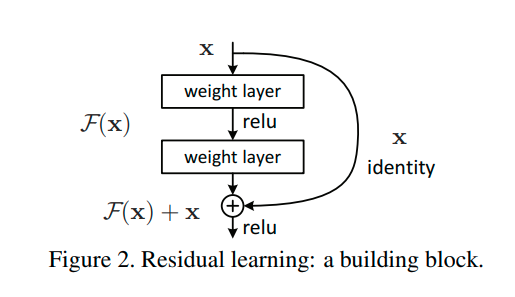
Source [Figure 2 - Deep Resual Learning for Image Recognition] Skip Connection (or shortcut connection) on ResNet block.

We assume that output of shallow learned layer is $\mathbf{x}$, the feed forward non-linear transform it into $\mathcal{F}(\mathbf{x})$. We hypothesize reality output of the whole process is $\mathcal{H}(\mathbf{x})$. So the residual between deeper layer compared with shallower layer is:

\[\mathcal{F}(\mathbf{x}; W_i) := \mathcal{H}(\mathbf{x}) - \mathbf{x}\]

$W_i$ are the model parameters in many convolutional layers of $\mathcal{F}$ transformation and also being to learn in backpropagation.

The learning process actually study non-linear transform $\mathcal{F}(\mathbf{x}; W_i)$ of residual after each block between input and output. It is going to be easier than learning non-linear transform input to output in directly way.

the skip connections simply perform identity mapping, and their outputs are added to the outputs of the stacked layers. So, we simply name it as indentity block.

The other block we applied convolutional transformation before skip connection from input layers to output layers in order to study feature learning.

\[\mathbf{y} = \mathcal{F}(\mathbf{x}; W_i) + \text{Conv}(\mathbf{x})\]

To keep output’s shape unchange and reduce the total parameters, $\text{Conv}$ layers normally have kernel size 1 x 1.

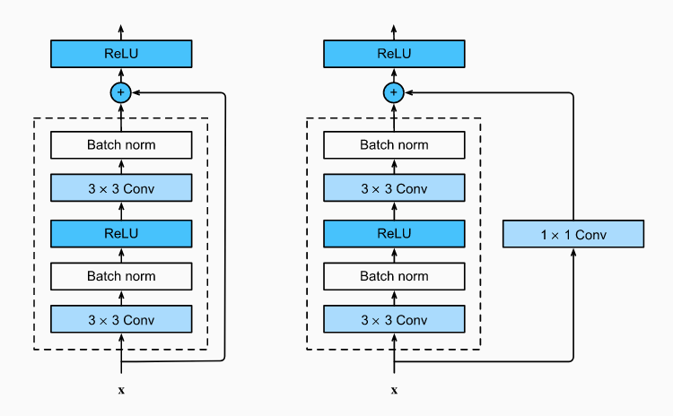
Source ResNet block with and without 1×1 convolution

3. How to build up Residual Block

After you firmly understand the general architecture of Residual Block, I introduce you to how can build up this fantastic block from scratch on three common deep learning frameworks. at the bellow, We design block to feed-forward input data in such a way enabling to control the output by adjusting strides argument in a block. For example, if you want to keep the same output shape, you set up strides = 1 and reduce twice time, you set up strides = 2. Besides, I facilitate you to practice on the colab notebook.

tensorflow

import tensorflow as tf

class ResidualBlockTF(tf.keras.layers.Layer):
  def __init__(self, num_channels, output_channels, strides=1, is_used_conv11=False, **kwargs):
    super(ResidualBlockTF, self).__init__(**kwargs)
    self.is_used_conv11 = is_used_conv11
    self.conv1 = tf.keras.layers.Conv2D(num_channels, padding='same', 
                                        kernel_size=3, strides=1)
    self.batch_norm = tf.keras.layers.BatchNormalization()
    self.conv2 = tf.keras.layers.Conv2D(num_channels, padding='same', 
                                        kernel_size=3, strides=1)
    if self.is_used_conv11:
      self.conv3 = tf.keras.layers.Conv2D(num_channels, padding='same', 
                                          kernel_size=1, strides=1)
    # Last convolutional layer to reduce output block shape.
    self.conv4 = tf.keras.layers.Conv2D(output_channels, padding='same',
                                        kernel_size=1, strides=strides)
    self.relu = tf.keras.layers.ReLU()

  def call(self, X):
    if self.is_used_conv11:
      Y = self.conv3(X)
    else:
      Y = X
    X = self.conv1(X)
    X = self.relu(X)
    X = self.batch_norm(X)
    X = self.relu(X)
    X = self.conv2(X)
    X = self.batch_norm(X)
    X = self.relu(X+Y)
    X = self.conv4(X)
    return X

X = tf.random.uniform((4, 28, 28, 1)) # shape=(batch_size, width, height, channels)
X = ResidualBlockTF(num_channels=1, output_channels=64, strides=2, is_used_conv11=True)(X)
print(X.shape)

(4, 14, 14, 64)

pytorch

import torch
from torch import nn

class ResidualBlockPytorch(nn.Module):
  def __init__(self, num_channels, output_channels, strides=1, is_used_conv11=False, **kwargs):
    super(ResidualBlockPytorch, self).__init__(**kwargs)
    self.is_used_conv11 = is_used_conv11
    self.conv1 = nn.Conv2d(num_channels, num_channels, padding=1, 
                           kernel_size=3, stride=1)
    self.batch_norm = nn.BatchNorm2d(num_channels)
    self.conv2 = nn.Conv2d(num_channels, num_channels, padding=1, 
                           kernel_size=3, stride=1)
    if self.is_used_conv11:
      self.conv3 = nn.Conv2d(num_channels, num_channels, padding=0, 
                           kernel_size=1, stride=1)
    # Last convolutional layer to reduce output block shape.
    self.conv4 = nn.Conv2d(num_channels, output_channels, padding=0, 
                           kernel_size=1, stride=strides)
    self.relu = nn.ReLU(inplace=True)
    
  def forward(self, X):
    if self.is_used_conv11:
      Y = self.conv3(X)
    else:
      Y = X
    X = self.conv1(X)
    X = self.relu(X)
    X = self.batch_norm(X)
    X = self.relu(X)
    X = self.conv2(X)
    X = self.batch_norm(X)
    X = self.relu(X+Y)
    X = self.conv4(X)
    return X

X = torch.rand((4, 1, 28, 28)) # shape=(batch_size, channels, width, height)
X = ResidualBlockPytorch(num_channels=1, output_channels=64, strides=2, is_used_conv11=True)(X)
print(X.shape)

torch.Size([4, 64, 14, 14])

mxnet

Google colab docker may be unavailable mxnet pakcage. In case of missing, you install very simple as bellow:

!pip install mxnet

Requirement already satisfied: mxnet in /usr/local/lib/python3.6/dist-packages (1.7.0.post1)
Requirement already satisfied: numpy<2.0.0,>1.16.0 in /usr/local/lib/python3.6/dist-packages (from mxnet) (1.19.4)
Requirement already satisfied: graphviz<0.9.0,>=0.8.1 in /usr/local/lib/python3.6/dist-packages (from mxnet) (0.8.4)
Requirement already satisfied: requests<3,>=2.20.0 in /usr/local/lib/python3.6/dist-packages (from mxnet) (2.23.0)
Requirement already satisfied: certifi>=2017.4.17 in /usr/local/lib/python3.6/dist-packages (from requests<3,>=2.20.0->mxnet) (2020.12.5)
Requirement already satisfied: urllib3!=1.25.0,!=1.25.1,<1.26,>=1.21.1 in /usr/local/lib/python3.6/dist-packages (from requests<3,>=2.20.0->mxnet) (1.24.3)
Requirement already satisfied: chardet<4,>=3.0.2 in /usr/local/lib/python3.6/dist-packages (from requests<3,>=2.20.0->mxnet) (3.0.4)
Requirement already satisfied: idna<3,>=2.5 in /usr/local/lib/python3.6/dist-packages (from requests<3,>=2.20.0->mxnet) (2.10)

import mxnet as mx
from mxnet.gluon import nn as mxnn

class ResidualBlockMxnet(mxnn.Block):
  def __init__(self, num_channels, output_channels, strides=1, is_used_conv11=False, **kwargs):
    super(ResidualBlockMxnet, self).__init__(**kwargs)
    self.is_used_conv11 = is_used_conv11
    self.conv1 = mxnn.Conv2D(num_channels, padding=1, 
                           kernel_size=3, strides=1)
    self.batch_norm = mxnn.BatchNorm()
    self.conv2 = mxnn.Conv2D(num_channels, padding=1, 
                           kernel_size=3, strides=1)
    if self.is_used_conv11:
      self.conv3 = mxnn.Conv2D(num_channels, padding=0, 
                           kernel_size=1, strides=1)
    self.conv4 = mxnn.Conv2D(output_channels, padding=0, 
                           kernel_size=1, strides=strides)
    self.relu = mxnn.Activation('relu')
    
  def forward(self, X):
    if self.is_used_conv11:
      Y = self.conv3(X)
    else:
      Y = X
    X = self.conv1(X)
    X = self.relu(X)
    X = self.batch_norm(X)
    X = self.relu(X)
    X = self.conv2(X)
    X = self.batch_norm(X)
    X = self.relu(X+Y)
    X = self.conv4(X)
    return X

X = mx.nd.random.uniform(shape=(4, 1, 28, 28)) # shape=(batch_size, channels, width, height)
res_block = ResidualBlockMxnet(num_channels=1, output_channels=64, strides=2, is_used_conv11=True)
# you must initialize parameters for mxnet block.
res_block.initialize()
X = res_block(X)
print(X.shape)

(4, 64, 14, 14)

As you can see, building the Residual Block is not quite hard with support of high level API on all frameworks: tensorflow keras, pytorch and mxnet gluon. They are all the same arrange of layers on the feed-forward process. Next step we shall deeply analyze of how to build up ResNet architectures under variate of model’s deepth options.

4. ResNet model

There are many kind of ResNet version changing by deepth. If you want to applied them on edge devices, you may concern to light weight ResNet18, ResNet34, ResNet50 models. In opposite aspect, you consider more about accuracy, computation resource is not a such big problem, i suggest you choose deeper models such as ResNet101, ResNet152.

Actually, in my current task related to label generation, i define to need one model that are good enough to make quality labels. Thus training another bigger model version that are separeted from my original model. Absolutely, bigger model is high computational cost and inappropriate to deploy on edge device.

4.1. Architecture of ResNet model

In generally, the common architecture of those different deepth ResNet models have the same rule. So, i introduce to you the analysis and the implementation of ResNet-18 architecture as such bellow description:

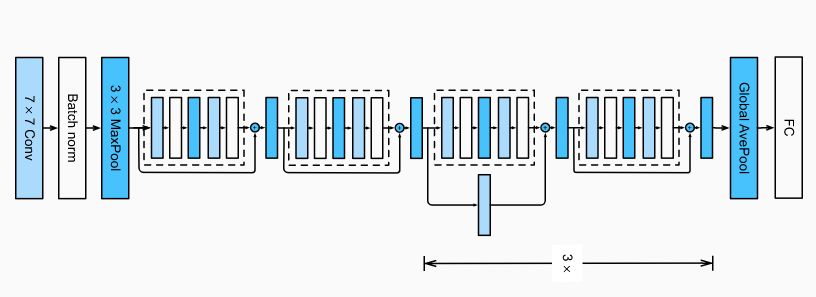
ResNet-18 architecture.

The starting layer is Convol2D 7 x 7, we choose bigger kernel size because of input shape is largest to capture features in the wider context. The coherent idea applied during the whole models that is the one batch normalization layer follow right behind each convolutional layer.

Residual block is enveloped by dash rectangle with 5 stacked layers in figure 3. The two starting residual blocks are identify blocks. After that, we repeat three times [convolutional mapping + identity mapping]. Finally, global average pooling applied to capture general features according to the deepth dimension and forward the final fully connected output.

Because of the repetation of residual blocks, we are going to neatly design the code to serve the general architecture in which only need to define each kind of block (indentity or convolution mapping) in each position. The sequential model module is the most prudent choice with such kind of stacked architecture.

4.2. Practice coding

I introduce to you three coding styles on tensorflow, pytorch, mxnet in order. They are share the same procedure. Through this practice, you facilitate to apply the given CNN architecture on any deep learning framework.

tensorflow

import tensorflow as tf

class ResNet18TF(tf.keras.Model):
  def __init__(self, residual_blocks, output_shape):
    super(ResNet18TF, self).__init__()
    self.conv1 = tf.keras.layers.Conv2D(filters=64, kernel_size=7, strides=2, padding='same')
    self.batch_norm = tf.keras.layers.BatchNormalization()
    self.max_pool = tf.keras.layers.MaxPool2D(pool_size=(3, 3), strides=2, padding='same')
    self.relu = tf.keras.layers.ReLU()
    self.residual_blocks = residual_blocks
    self.global_avg_pool = tf.keras.layers.GlobalAvgPool2D()
    self.dense = tf.keras.layers.Dense(units=output_shape)

  def call(self, X):
    X = self.conv1(X)
    X = self.batch_norm(X)
    X = self.relu(X)
    X = self.max_pool(X)
    for residual_block in residual_blocks:
      X = residual_block(X)
    X = self.global_avg_pool(X)
    X = self.dense(X)
    return X

residual_blocks = [
    # Two start conv mapping
    ResidualBlockTF(num_channels=64, output_channels=64, strides=2, is_used_conv11=False),
    ResidualBlockTF(num_channels=64, output_channels=64, strides=2, is_used_conv11=False),
    # Next three [conv mapping + identity mapping]
    ResidualBlockTF(num_channels=64, output_channels=128, strides=2, is_used_conv11=True),
    ResidualBlockTF(num_channels=128, output_channels=128, strides=2, is_used_conv11=False),
    ResidualBlockTF(num_channels=128, output_channels=256, strides=2, is_used_conv11=True),
    ResidualBlockTF(num_channels=256, output_channels=256, strides=2, is_used_conv11=False),
    ResidualBlockTF(num_channels=256, output_channels=512, strides=2, is_used_conv11=True),
    ResidualBlockTF(num_channels=512, output_channels=512, strides=2, is_used_conv11=False)
]

tfmodel = ResNet18TF(residual_blocks, output_shape=10)
tfmodel.build(input_shape=(None, 28, 28, 1))
tfmodel.summary()

pytorch

import torch
from torch import nn
from torchsummary import summary

class ResNet18PyTorch(nn.Module):
  def __init__(self, residual_blocks, output_shape):
    super(ResNet18PyTorch, self).__init__()
    self.conv1 = nn.Conv2d(in_channels=1, out_channels=64, kernel_size=7, stride=2, padding=3)
    self.batch_norm = nn.BatchNorm2d(64)
    self.max_pool = nn.MaxPool2d(kernel_size=3, stride=2, padding=1)
    self.relu = nn.ReLU()
    self.residual_blocks = nn.Sequential(*residual_blocks)
    self.global_avg_pool = nn.Flatten()
    self.dense = nn.Linear(in_features=512, out_features=output_shape)

  def forward(self, X):
    X = self.conv1(X)
    X = self.batch_norm(X)
    X = self.relu(X)
    X = self.max_pool(X)
    X = self.residual_blocks(X)
    X = self.global_avg_pool(X)
    X = self.dense(X)
    return X

residual_blocks = [
    # Two start conv mapping
    ResidualBlockPytorch(num_channels=64, output_channels=64, strides=2, is_used_conv11=False),
    ResidualBlockPytorch(num_channels=64, output_channels=64, strides=2, is_used_conv11=False),
    # Next three [conv mapping + identity mapping]
    ResidualBlockPytorch(num_channels=64, output_channels=128, strides=2, is_used_conv11=True),
    ResidualBlockPytorch(num_channels=128, output_channels=128, strides=2, is_used_conv11=False),
    ResidualBlockPytorch(num_channels=128, output_channels=256, strides=2, is_used_conv11=True),
    ResidualBlockPytorch(num_channels=256, output_channels=256, strides=2, is_used_conv11=False),
    ResidualBlockPytorch(num_channels=256, output_channels=512, strides=2, is_used_conv11=True),
    ResidualBlockPytorch(num_channels=512, output_channels=512, strides=2, is_used_conv11=False)
]

device = torch.device("cuda" if torch.cuda.is_available() else "cpu")

ptmodel = ResNet18PyTorch(residual_blocks, output_shape=10)
ptmodel.to(device)
summary(ptmodel, (1, 28, 28))

mxnet

import mxnet as mx
from mxnet.gluon import nn as mxnn

class ResNet18Mxnet(mxnn.Block):
  def __init__(self, residual_blocks, output_shape, **kwargs):
    super(ResNet18Mxnet, self).__init__(**kwargs)
    self.conv1 = mxnn.Conv2D(channels=64, padding=3, 
                           kernel_size=7, strides=2)
    self.batch_norm = mxnn.BatchNorm()
    self.max_pool = mxnn.MaxPool2D(pool_size=3)
    self.relu = mxnn.Activation('relu')
    self.residual_blocks = residual_blocks
    self.global_avg_pool = mxnn.GlobalAvgPool2D()
    self.dense = mxnn.Dense(units=output_shape)
    self.blk = mxnn.Sequential()
    for residual_block in self.residual_blocks:
      self.blk.add(residual_block)
  
  def forward(self, X):
    X = self.conv1(X)
    X = self.batch_norm(X)
    X = self.relu(X)
    X = self.max_pool(X)
    X = self.blk(X)
    X = self.global_avg_pool(X)
    X = self.dense(X)
    return X

residual_blocks = [
    # Two start conv mapping
    ResidualBlockMxnet(num_channels=64, output_channels=64, strides=2, is_used_conv11=False),
    ResidualBlockMxnet(num_channels=64, output_channels=64, strides=2, is_used_conv11=False),
    # Next three [conv mapping + identity mapping]
    ResidualBlockMxnet(num_channels=64, output_channels=128, strides=2, is_used_conv11=True),
    ResidualBlockMxnet(num_channels=128, output_channels=128, strides=2, is_used_conv11=False),
    ResidualBlockMxnet(num_channels=128, output_channels=256, strides=2, is_used_conv11=True),
    ResidualBlockMxnet(num_channels=256, output_channels=256, strides=2, is_used_conv11=False),
    ResidualBlockMxnet(num_channels=256, output_channels=512, strides=2, is_used_conv11=True),
    ResidualBlockMxnet(num_channels=512, output_channels=512, strides=2, is_used_conv11=False)
]

mxmodel = ResNet18Mxnet(residual_blocks, output_shape=10)
mxmodel.hybridize()

mx.viz.print_summary(
    mxmodel(mx.sym.var('data')), 
    shape={'data':(4, 1, 28, 28)}, #set your shape here
)

5. Train model

After build up the model, train model is the simple step. In this step i take an example how to train classify digits on mnist dataset. There are total 10 different classes corresponding with digits from 0 to 9. The input is picture with shape 28 x 28 x 1. Dataset is splitted into train:test with proportion 10000:60000 and distribution of data is equal between all classes at both train and test.

tensorflow

Training model on tensorflow keras is wrapped in fit() function. Thus, it seem to be simpliest in 3 deep learning frameworks. You can see as below:

import tensorflow as tf
from tensorflow.keras.datasets import mnist
import numpy as np

(X_train, y_train), (X_test, y_test) = mnist.load_data()
X_train = X_train/255.0
X_test = X_test/255.0
X_train = np.reshape(X_train, (-1, 28, 28, 1))
X_test = np.reshape(X_test, (-1, 28, 28, 1))
# Convert data type bo be adaptable to tensorflow computation engine
y_train = y_train.astype(np.int32)
y_test = y_test.astype(np.int32)
print(X_test.shape, X_train.shape)

(10000, 28, 28, 1) (60000, 28, 28, 1)

Train model

from tensorflow.keras.optimizers import Adam
opt = Adam(lr=0.001, beta_1=0.9, beta_2=0.99)
tfmodel.compile(optimizer=opt, loss=tf.keras.losses.SparseCategoricalCrossentropy(from_logits=True), metrics=['accuracy'])
tfmodel.fit(X_train, y_train,
            validation_data = (X_test, y_test), 
            batch_size=32,
            epochs=10)

pytorch

On the pytorch you are going to see there are a little bit change compare to tensorflow keras training. You normally use DataLoader to forward training. It is very through bellow practice.

import torch.optim as optim
import torch
import torchvision
import torchvision.transforms as transforms
import time

device = torch.device("cuda" if torch.cuda.is_available() else "cpu")

transform = transforms.Compose(
    [transforms.ToTensor(),
     transforms.Normalize((0.05), (0.05))])

trainset = torchvision.datasets.MNIST(root='./data', train=True,
                                        download=True, transform=transform)
trainloader = torch.utils.data.DataLoader(trainset, batch_size=32,
                                          shuffle=True, num_workers=8)

testset = torchvision.datasets.MNIST(root='./data', train=False,
                                       download=True, transform=transform)
testloader = torch.utils.data.DataLoader(testset, batch_size=32,
                                         shuffle=False, num_workers=8)

criterion = nn.CrossEntropyLoss()
optimizer = optim.Adam(ptmodel.parameters(), lr=0.001, betas=(0.9, 0.99))

                        
def acc(output, label):
    # output: (batch, num_output) float32 ndarray
    # label: (batch, ) int32 ndarray
    return (torch.argmax(output, axis=1)==label).float().mean()

for epoch in range(10):  # loop over the dataset multiple times
    total_loss = 0.0
    tic = time.time()
    tic_step = time.time()
    train_acc = 0.0
    valid_acc = 0.0
    for i, data in enumerate(trainloader, 0):
        # get the inputs; data is a list of [inputs, labels]
        inputs, labels = data
        inputs, labels = inputs.to(device), labels.to(device)

        # zero the parameter gradients
        optimizer.zero_grad()

        # forward + backward + optimize
        outputs = ptmodel(inputs)
        train_acc += acc(outputs, labels)
        loss = criterion(outputs, labels)
        loss.backward()
        optimizer.step()

        # print statistics
        total_loss += loss.item()
        if i % 500 == 499:
          print("iter %d: loss %.3f, train acc %.3f in %.1f sec" % (
            i+1, total_loss/i, train_acc/i, time.time()-tic_step))
          tic_step = time.time()

    # calculate validation accuracy
    for i, data in enumerate(testloader, 0):
        inputs, labels = data
        inputs, labels = inputs.to(device), labels.to(device)

        valid_acc += acc(ptmodel(inputs), labels)

    print("Epoch %d: loss %.3f, train acc %.3f, test acc %.3f, in %.1f sec" % (
            epoch, total_loss/len(trainloader), train_acc/len(trainloader),
            valid_acc/len(testloader), time.time()-tic))

print('Finished Training')

mxnet

To train model on mxnet also the same as pytorch, we also loop through DataLoader to forward and backpropagation.

from mxnet import nd, gluon, init, autograd, gpu, cpu
from mxnet.gluon import nn
from mxnet.gluon.data.vision import datasets, transforms
import matplotlib.pyplot as plt
import time

mnist_train = datasets.MNIST(train=True)
mnist_val = datasets.MNIST(train=False)

transformer = transforms.Compose([
    transforms.ToTensor(),
    transforms.Normalize(0.05, 0.05)])

mnist_train = mnist_train.transform_first(transformer)
mnist_val = mnist_val.transform_first(transformer)

Downloading /root/.mxnet/datasets/mnist/t10k-images-idx3-ubyte.gz from https://apache-mxnet.s3-accelerate.dualstack.amazonaws.com/gluon/dataset/mnist/t10k-images-idx3-ubyte.gz...
Downloading /root/.mxnet/datasets/mnist/t10k-labels-idx1-ubyte.gz from https://apache-mxnet.s3-accelerate.dualstack.amazonaws.com/gluon/dataset/mnist/t10k-labels-idx1-ubyte.gz...

batch_size = 32
train_data = gluon.data.DataLoader(
    mnist_train, batch_size=batch_size, shuffle=True, num_workers=4)
valid_data = gluon.data.DataLoader(
    mnist_val, batch_size=batch_size, shuffle=True, num_workers=4)

To train model of mxnet on GPU, you should install mxnet-cuda version aligning with your computer cuda version.

# check cuda version
!nvcc --version
# install mxnet-cuda version
!pip install mxnet-cu101

nvcc: NVIDIA (R) Cuda compiler driver
Copyright (c) 2005-2019 NVIDIA Corporation
Built on Sun_Jul_28_19:07:16_PDT_2019
Cuda compilation tools, release 10.1, V10.1.243
Collecting mxnet-cu101

use_gpu = True
if use_gpu:
  # incase you have more than one GPU, you can add gpu(1), gpu(2),...
  devices = [gpu(0)]
else:
  devices = [cpu()]
print('devices: ', devices)
mxmodel = ResNet18Mxnet(residual_blocks, output_shape=10)
mxmodel.hybridize()
mxmodel.collect_params()
mxmodel.initialize(init=init.Xavier(), ctx=devices, force_reinit=True)
softmax_cross_entropy = gluon.loss.SoftmaxCrossEntropyLoss()
trainer = gluon.Trainer(mxmodel.collect_params(), 'adam', {'learning_rate': 0.001})
                        
def acc(output, label):
    # output: (batch, num_output) float32 ndarray
    # label: (batch, ) int32 ndarray
    return (output.argmax(axis=1) ==
            label.astype('float32')).mean().asscalar()

for epoch in range(10):
    train_loss, train_acc, valid_acc = 0., 0., 0.
    tic = time.time()
    for i, (inputs, labels) in enumerate(train_data):
        actual_batch_size = inputs.shape[0]
        # Split data among GPUs. Since split_and_load is a deterministic function
        # inputs and labels are going to be split in the same way between GPUs.
        inputs = mx.gluon.utils.split_and_load(inputs, ctx_list=devices, even_split=False)
        labels = mx.gluon.utils.split_and_load(labels, ctx_list=devices, even_split=False)
        with mx.autograd.record():
          for input, label in zip(inputs, labels):
            output = mxmodel(input)
            loss = softmax_cross_entropy(output, label)

        loss.backward()
        # update parameters
        trainer.step(batch_size)
        # calculate training metrics
        train_loss += loss.mean().asscalar()
        train_acc += acc(output, label)
        if i % 500 == 499:
          print("Epoch %d: Step %d: loss %.3f, train acc %.3f" % (
              epoch, i+1, train_loss/i, train_acc/i))
    # calculate validation accuracy
    for inputs, labels in valid_data:
        actual_batch_size = inputs.shape[0]
        # Split data among GPUs. Since split_and_load is a deterministic function
        # inputs and labels are going to be split in the same way between GPUs.
        inputs = mx.gluon.utils.split_and_load(inputs, ctx_list=devices, even_split=False)
        labels = mx.gluon.utils.split_and_load(labels, ctx_list=devices, even_split=False)
        for input, label in zip(inputs, labels):
          output = mxmodel(input)
          valid_acc += acc(output, label)

    print("Epoch %d: loss %.3f, train acc %.3f, test acc %.3f, in %.1f sec" % (
            epoch, train_loss/len(train_data), train_acc/len(train_data),
            valid_acc/len(valid_data), time.time()-tic))

Through this blog, i introduce to you how to initialize ResNet model from scratch on the whole 3 most common deep learning frameworks. You can realize that when you understand about model architecture, you can easily build up model and customize it according to your new ideas to improve it better and better.

If you see this blog is useful, kindly subcribe my channels via phamdinhkhanh, Khanh Blog and AICode.

Lesson 53 - ResNet model

1. ResNet history

2. General Architecture

2.1. Batch Normalization

2.2. Skip Connection

3. How to build up Residual Block

4. ResNet model

4.1. Architecture of ResNet model

4.2. Practice coding

5. Train model

6. Referrence