1. StarGAN Multi-Domain Image-to-Image translation

In previous sections, you are introduced about::

• pix2pix GAN is a kind of conditional GAN that you enable to control desired output. The loss function is the combination of adversarial loss and L1-loss. To train pix2pix GAN required to couple source and target images. So it is low performance on small and scarce dataset.

• CycleGAN that is unsupervised GAN model enable to learn how to translate from one source dataset to another target dataset. CycleGAN is high performance and more realistic image generation than pix2pix because of it bases on the dataset instead of only each pair image. The model using cycle consistent loss function beside adversarial loss. The cycle consistent loss function is a greate creation that empower CycleGAN to auto-encode the image itself through finding out the efficient latent space that good present the $x$ input image to $y$ output image. It is pretty well studies on the small dataset without coupling image. But you only have ability to train to transfer unique domain. Such as transfer color from hourse to zibra, from colored images to sketch images or from dark to night.

But how can we handle if we want to Multi-Domain translate from source to target. For example, you have a face dataset owning variety of features such as age, gender, hair color, skin face color, facial expression,…. Previous GAN like pix2pix and CycleGAN models only support to translate one feature. For example, you only enable to translate from male to female or change age from young to old. With each needed-translating feature, you have to train seperate model. Thus if you have $k$ distinct features, to transfer two features simultaneously you may develop $k \times (k-1)$ GAN models. This is highly consuming cost and inefficient. Thus that is the reason to clova’s AI researchers create StarGAN model to handle with problem of Multi-Domain in image-to-image translation. Replacing $k \times (k-1)$ distinctive models by unique StarGAN model that is capable to learn every translation of many features through binary-encoding domain vector and input image. It is fascinating and interesting mechanism that today, we are going to discover the secret mechanism inside it.

2. How to learn Multi-Domain feature

2.1. Problem when cross-domain

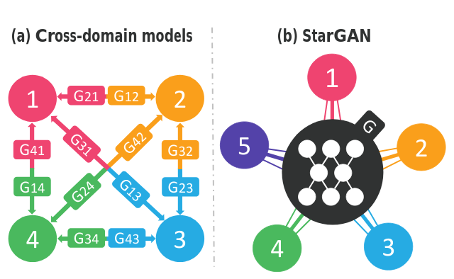
You can see in image below, the cross-domain model (on the left) is only map between one to one feature. Hence, when there are four distinctive features indexed as $1, 2, 3, 4$, you have to build 12 generative model in total to cover whole translation. Such as to translate the feature 1->2 is $G_{12}$ model and 2->1 is $G_{21}$ model. It also mean that if you want to translate color of hair from brown to black, there is a new model is developed and to inverse translate from black to brown, there is another one is developed.

But StarGAN on the right of the bellow image empowers to you only use unique generator architecture that is more powerful and flexiable when support to translation of multi-domain features at once. You not only translate hair color but also aligned translate with the other features such as gender or age.

2.2. StarGAN architecture

So how does the StarGAN architecture look like?

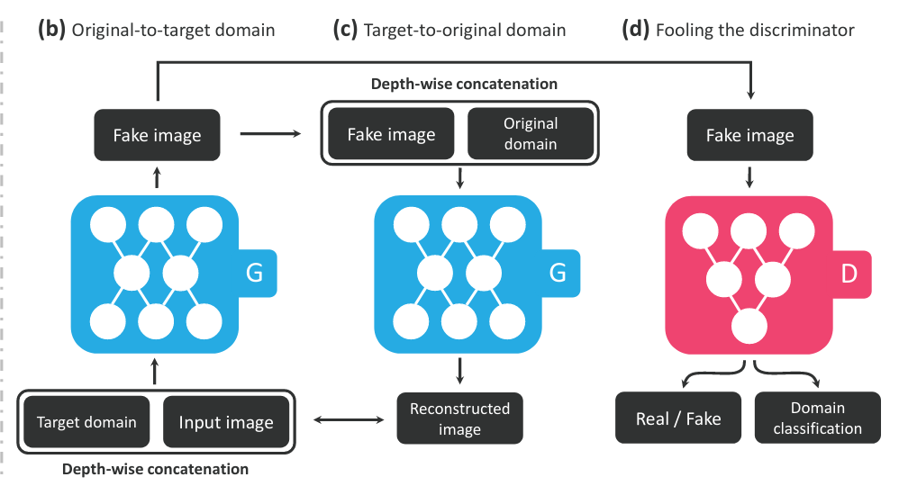
Model take target domain as embedding vector of condition. The idea is natural as in conditional GAN, when you want what the features are going to appear on the output, you must add condition label to input beside the input image.

Abve is StarGAN generator graphic.

• At the (b) step Original-to-target domain: Generator take both target domain and input image as the input. Target domain is binary-encoded to force generator to intentionally create the fake image with specific features. The target domain is spatially expanded to feasibly combine into input image add the new channels.

• (c) Target-to-original domain: After step b, the fake image own the characteristic of target domain. Next, in this c step we start reconstruction process that convert target to original domain. the fake image is depth-wise concatenation with original domain to have ability to reconstruct the original features and thus, reconstruct into the original image. The whole reconstruction proccess we applied the second generator architecture that is somehow similar to CycleGAN.

• (d) Fooling the discriminator: The discriminator after that is discriminated by discriminator. Because we not only try to create the fake image, the features is also what we want to create. Hence the discriminator is bound to classify both real/fake image and domain classification. Is that easy? I hope you understood.

As ussual in the almost training discriminator, we align fake case with real case to feed into model.

Finally, model find the balance point that makes a good generator and discriminator to generate output images as realistic as possible.

2.3. Mask Vector for Domain classification

On StarGAN we train model on multi-dataset. Each dataset can own some feature that is not defined on the other dataset. For example, when we train StarGAN with face, on both CelebA and RaFD dataset. The image originates from CelebA we only have blond hair, gender, age, pale skin but do not have information about angry, happy, and fearful that defined on RaFD and vice verse. So we must apply the mask vector which forces the model to forget the features that do not have. Mask vector is exactly binary vector that encode 1 value if feature is exist and 0 in the other hand.

For example: You have 7 features

• blond hair: yes/no
• gender: male 1, female 0
• age: old 1, young 0
• pale skin: yes/no
• angry: yes/no
• happy:yes/no
• fearful: yes/no

yes correspond with 1 and no correspond with 0.

With one face image from CelebA it own features: blond hair, female, young, no pale skin. So it may be encoded as [1, 0, 0, 0, 0, 0, 0] that allow the order of 7 features we list above. The only CelebA’s features must be defined, the RaFD’s features is forgot.

3. The loss function

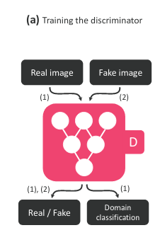
The target of StarGAN is to discriminate real and fake image and classify the domain belonging to each input image. Thus discriminator return the distribution outputs include both probability of source distribution $D_{src}$ (for distingushing real/fake image) and domain distribution $D_{cls}$ (for classifying multi-domain).

3.1. Adversarial Loss

The main adversarial loss’s role is to distingush better between real and fake image. Thus, it imposes on the source distribution $D_{src}$. It actually is the kind of binary cross-entropy loss function. In which we consider the both cases contribute to loss is $y=0$ and $y=1$.

$G(z, c)$ is generator suppose to generate the fake image on step (b) you see. Because of model consider the fake case as negative, hence the contribution to loss function must be $1 - \log D_{src}(G(z, c))$. And in opposite, the real case contribution must be $\log D_{src}(x)$.

1
2
3
4
5
6
7
8
9
10
11
12
13
14
15
import torch
import torch.nn.functional as F

def adv_loss(logits, target):
    """
    logits: source probability output of discriminator.
    target: target label of fake image. 1 as real and 0 as fake
    """
    targets = torch.full_like(logits, fill_value=target)
    loss = F.binary_cross_entropy_with_logits(logits, targets)
    return loss

logits = torch.tensor([0.1])
target = 1
adv_loss(logits, target)

1
tensor(0.6444)

3.2. Domain Loss

Domain Loss simply serves to optimize the Multi-Domain classification problem. The labels that Multi-Domain classifier need to predict is the target domain features of fake image or the real features from real image. In generally, Domain Loss function allowed the form crossentropy loss function:

In which $D_{cls}(c|x)$ is the probability value belonging to class $c$ when the input is $x$.

In case the image is real or fake also change the domain loss representation above. Intuitively, it must be:

• Domain Loss Function for real image:

• Domain Loss Function for fake image: The real value $x$ is replaced by output of generator $G$.

1
2
3
4
5
6
7
8
9
10
11
12
13
14
15
16
17
18
19
20
import torch

def domain_loss(d_out, c):
  """
  d_out: the output of descriminator
  c: features index that fake image own.
  """
  # one-hot encoding
  v_out = torch.full_like(d_out, 0)
  v_out[c] = 1
  # loss function
  loss = -v_out*torch.log(d_out)
  loss=loss.sum()
  return loss

rand = torch.randn(4)
d_out = torch.exp(rand)/torch.exp(rand).sum()
c = torch.tensor([1, 2])

domain_loss(d_out, c)

1
tensor(1.5890)

3.3. Reconstruction Loss

The step (b) and (c) is also very similiar to what happen in CycleGAN. In which output of process is the reconstruction of input image. We do not guarantee after applying Multi-domain translation on input image, the output is going keep the patterns of the input image. To alleviate the diffrence too much, we apply the kind of Cycle Consistency Loss under the L1-norm formulation:

In which $G_1$ is first generator that applied on step (b) to create fake image replying on the input $x$ and target class labels $c_t$. Then, the fake image $G_1(x, c_t)$ and added source class labels $c_{org}$ continues forwarding on $G_2$ second generator to reconstruct back to original input image.

We call this loss function as reconstruction loss to remind the recovery aim of this specical loss function.

1
2
3
4
5
6
7
8
9
10
import torch

def rec_l1(x, g_out):
  assert x.size() == g_out.size()
  return torch.mean(torch.abs(x-g_out))

x = torch.randn((4, 28, 28, 3))
g_out = torch.randn((4, 28, 28, 3))

_rec_l1(x, g_out)

1
tensor(1.1204)

3.4. Full Objective Function

The full objective function is the combination of three above kinds of loss function. They are relatively assigned to loss function of discriminator and generator as bellow:

You might ask to why the sign of $\mathcal{L}_{adv}$ on generator loss? It is simple that when your generator is good enough, it intentionally create image approach to real. Thus, $D_{cls}(G(z, c))$ is approach to $1$ and that is reason cause to $\mathcal{L}_{adv}$ is high. We revert the sign of it on generator to be adaptable with our target is to minimize loss function.

Beside, $\lambda_{cls}, \lambda_{rec}$ are graduately two hyper-parameters of model that control the importance of domain classification and reconstruction impact on full objective loss relatively. In emperically, we choose $\lambda_{cls}=1$ and $\lambda_{rec}=10$.

4. Source code

• Pytorch:

https://github.com/yunjey/stargan

https://github.com/clovaai/stargan-v2

https://github.com/eveningglow/StarGAN-pytorch

• Tensorflow:

https://github.com/taki0112/StarGAN-Tensorflow

https://github.com/clovaai/stargan-v2-tensorflow

https://github.com/KevinYuimin/StarGAN-Tensorflow

5. Conclusion

Through this lesson, i introduce to you the main keypoints of StarGAN that make this model get high performance. Especially it have ability to Multi-Domain translating images that help to cost saving when required unique generator but apply variety translations. StarGAN own this extraodinary ability is depending on embedding features multi-domain features and align them with image as additional condition for inferencing.

I hope you enjoy with this content and thanks for reading.

6. Reference

1. StarGAN: Unified Generative Adversarial Networks for Multi-Domain Image-to-Image Translation
2. CycleGAN - Khanhblog
3. Pix2PixGAN - Khanhblog
4. Conditional GAN - Khanhblog
5. Wasserstein GAN - Khanhblog