
Lesson 54 - CycleGAN Unpaired image to image translation
20 Jan 2021 - phamdinhkhanh1. Introduction
In reality, there are many image to image translation tasks such as:
- Transforming image color between two pictures.
- Changing season from summer to winter.
- Changing dark to night and night to dark.
- Transforming colored images into sketch images.
- Translating hourse into zebra.
- Translating photo into the painting of the dead artists.
When face up with these tasks related to image to image translation, CycleGAN may be the best facility you should think first.
CycleGAN was launched in 2017 by group author Jun-Yan Zhu, Taesung Park, Phillip Isola, Alexei A. Efros. That model find the general way to map between input images to output images without aligning the pair of source and target like the other GAN models such as Pix2Pix and CGAN. So the results gain from CycleGAN is more general when it can learn not only from source image to target image but also learn inter-domain mapping from a set of source images to target images. This model is especially useful when model is trained on scarce images that is hard to couple. Because of lacking of data, we are not easily to learn and transfer characteristic from only source image to target image. That kind of learning is unsupervised learning through unpaired data.
1.1. Unpaired learning image to image translation
We all known the normal GAN models have input is paired. That make an disavantage to model get high performance of generalization and synthesis ability. Usually model need a large scale dataset to reach generating the fake image as real. But there are some data is scarce and hard to be found, for example: the pictures from the dead artist.
To overcome this disavantage, The CycleGAN’s authors introduce unpaired image to image translation learning that supports translating the general characteristics from source to target set without requiring them related to in pair.
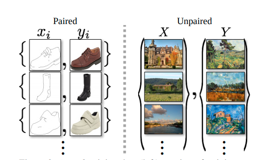
Figure 1: Paired (in the left) vs Unpaired (in the right) image to image translation. Paired training dataset exists the correspondance of each input image $x_i$ and $y_i$. In contrast, unpaired training dataset have input is both sets $X = \set{ x_i }^{M}_{i=1}$
and $Y=\set{ y_i }^{M}_{i=1}$ with no information of mapping $x_i$ to $y_i$ inside them.
Because of unpair source-target couple, we do not exactly know what the specific source image maps to target image. But in the other hand, model learn mapping at the set level between set $X$ to set $Y$ under the unsupervised learning. The process of training corresponds with find a mapping function $G: X \mapsto Y$. We expect that the output is indistinguishable with real image, so the distribution of each image $x \in X$ require $\hat{y} = G(x)$ is identical with $y \in Y$ and the distribution of $G(X)$ set may have to be approach to the distribution of $Y$ set. The mapping function $G$ is definitely the generator function. To train generator function, we use discriminator function help to distinguish between real and fake image.
2. CycleGAN architecture
2. 1. Different between CycleGAN and GAN architecture
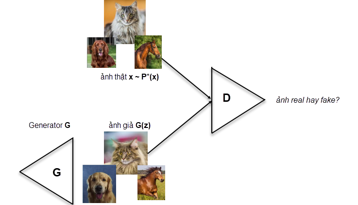
Figure2: Normal GAN architecture. Firstly, input noise vector $z$ is transform into cenerator to create fake image. discriminator help to distinguish between real/ fake data.
GAN model is optimized on adversarial loss function which is the combination between generator loss and discriminator loss.
\[\min_{G} \max_{D} V(D, G) = \underbrace{\mathbb{E}_{x \sim p_{data}(x)} [\log D(x)]}_{\text{log-probability that D predict x is real}} + \underbrace{\mathbb{E}_{z \sim p_{z}(z)} [\log (1-D(G(z)))]}_{\text{log-probability D predicts G(z) is fake}} ~~~ (1)\]You should understand this loss function through my explanation at adversarial loss function of GAN. Kindly try to google translate if you are not Vietnamese.
In brief, that loss function not only discriminate between real and fake data and but also learn generate fake image more realistic. But in practical, it is really hard to train only adversarial objective because of divergence and unstability. The results also is not quite good.
` Moreover, in practice, we have found it difficult to optimize the adversarial objective in isolation: standard procedures often lead to the well known problem of mode collapse, where all input images map to the same output image and the optimization fails to make progress. `
Source Unpaired Image-to-Image Translation using Cycle-Consistent Adversarial Networks
Thus, CycleGAN authors come up with new architecture that allow to learn from both $X$ and $Y$ set without coupling the source and target image.
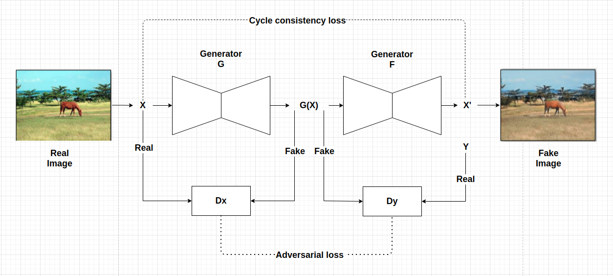
Figure3: CycleGAN architecture includes two generators and discriminatorS serve to translation from $X$ to $Y$ and opposite $Y$ to $X$.
This architecture also include generator and discriminator as the GAN architectures with the commission of each as bellow:
- generator: Try to generate real image look realistic as possible.
- discriminator: Improving generator through trying to discriminate real vs fake image (fake image come from generator).
But three are some improvements of CycleGAN architecture than GAN:
-
We use dual generator in continous to translate $x$ to $y$ and next restrain back $y$ to $x$. This architecture create a latent space to transform image without predefine paired image.
-
Cycle consistency loss function is applied to keep distribution of output of dual generator process not far from input.
Finally, the loss function is combination of cycle consistency loss and adversarial loss.
In the next section, i explain detail more about the CycleGAN through cycle consistency loss function. code
2.2. Cycle consistency loss function
To overcome the hardship of collapsion when train GAN model, CycGAN propose a cycle consistency loss function that learning in both direction starting from $X$ and $Y$. We suppose another inverse function of $G$, assuming $F$ to support mapping from $Y$ set to $X$ set. That invention is proved to keep dominance to the other algorithm in image to image translation replying on hand-defined factorizations or shared embedding functions.
As you see in figure 3, there are two generator function include $G$ on the left and $F$ in the right. $G$ help to generate $X \mapsto Y$ and $F$ is inversed $Y \mapsto X$. The output $G(x) \approx y$ and being continued to forward as input of $F$. This process in brief as
\[x \mapsto G(x) \mapsto F(G(x)) \approx x \tag{2}\]And in the revert direction, we change $y$ as $x$ to get process
\[y \mapsto F(y) \mapsto G(F(y)) \approx y \tag{3}\]Cycle consistency loss function try to constrain both of these $(2)$ and $(3)$ processes to it generate output become as real as possible. It corresponds with minimizing the difference between $F(G(x))-y$ and $G(F(x))-y$ reply on L1-norm as following:
\[\mathcal{L}_{cyc(G, F)} = \mathbb{E}_{x\sim p_{data}(x)} [||F(G(x)) − x||_1] + \mathbb{E}_{y\sim p_{data}(y)} [||G(F(y)) − y||_1]\]The cycle in cycle consistency loss meaning that the learning process repeats in both direction from $x$ and $y$.
2.3. Adversarial loss function
Adversarial loss function is totally the same as $(1)$ formulation. The aim of adversarial loss is to try simultaneously support generator generate fake image more realistic and increase discrimination capability between real and fake of discriminator.
There are two process of training as in $(2), (3)$ in the cycleGAN. Thus, there are also exist two adversarial loss functions corresponding with each of them.
- Start from $x$ we try to generate fake $\hat{y}=G(x)$.
- And in the revert direction, start from $y$: we try to fake $\hat{x}=F(y)$.
2.4. Training strategy
To training process stable, authors replace the negative log likelihood function $\mathcal{L}_{\text{GAN}}$ by least-square loss.
For example $\mathbb{E}_{y \sim p_{\text{data}}(y) }[\log D_{Y} (y)]$ is replaced by $\mathbb{E}_{y \sim p_{\text{data}}(y)}[(D_{Y} (y))^2]$
and $\mathbb{E}_{x \sim p_{data}(x)}[\log(1 − D_{Y} (G(x))]$ is replaced by $\mathbb{E}_{x \sim p_{data}(x)}[(1 − D_{Y} (G(x)))^2]$.
In emperical, this way is more efficient when generate image with high quality. $\lambda$ also set 10 is good. To reduce model oscillation, the descriminator is updated base on buffer of 50 history images instead of only lastest generator image.
Finally, we got the full objective function is summation of cycle consistency loss and adversarial loss.
The training stategy is process of found the optimization:
\[G^{∗}, F^{∗} = \arg \min_{G,F} \max_{ D_X,D_Y} \mathcal{L}(G, F, D_X, D_Y )\]maximization is to reinforce the strength of discriminator $D_X, D_Y$ through negative log likelihood function (or cross entropy in the other name). minimization is reply on $G, F$ function, that try to gain the most precise mapping function to create fake image as real.
Actually, we can consider model are learning autoencoder $G \circ F$ and $F \circ G$ jointly. One image is mapped to it-self via an intermediate representation similiar to bottle neck layer function in autoencoder.
3. Backbone
3.1. Generator
The generator of CycleGAN is the convolution-deconvolution network that usually is applied in image to image translation task. In detail, the network contains three convolutions block to reduce the resolution twice time at each layer at the beginning stage. Next, we keep the resolution the same on the next 6 blocks, this is to transform these features to get the fine-grained these features at the end. And on the deconvolution, we use transpose convolution to upsampling the output twice time until we meet the original resolution. I brief those architecture as bellow figure.
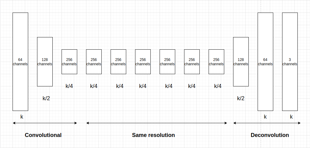
Figure4: Generator architecture include Convolutional and Deconvolutional phases. The resolution and channels are keep as above figure.
3.2. Discriminator
In discriminator, the author use 70x70 patchGAN architecture to classify on each small patch, the combination of whole patches make the final result of discriminator more trusted. Such patch-level discriminator architecture also has fewer parameters than full-image discriminator.
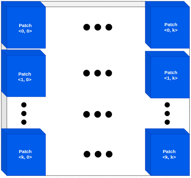
Figure5: PatchGAN architecture, the classification result is on each patch as on the figure.
About patchGAN i refer you to PatchGAN in pix2pix.
4. Code
The coding of cycleGAN you can find in many sources:
- pytorch:
https://github.com/junyanz/pytorch-CycleGAN-and-pix2pix/
https://github.com/aitorzip/PyTorch-CycleGAN
https://github.com/yunjey/mnist-svhn-transfer
- tensorflow:
https://github.com/LynnHo/CycleGAN-Tensorflow-2
https://www.tensorflow.org/tutorials/generative/cyclegan
- mxnet:
https://github.com/junyanz/CycleGAN
https://github.com/Ldpe2G/DeepLearningForFun/tree/master/Mxnet-Scala/CycleGAN
5. Conclusion
CycleGAN is kind of unsuppervised GAN model learning translation from set $X$ to $Y$ without pre-defining the pair <source, target> images. CycleGAN usually used on these tasks related to image to image translation such as color transfering, object transfiguration. This architecture uses cycle consistency loss function enable to learn on both direction from set $X$ to $Y$ and reverse $Y$ to $X$. Through this paper, I help you clear the keypoints make CycleGAN is efficient than previous GAN architectures. Thus, you can apply CycleGAN on task such as image to image translation without ambigous understood.